Your cart is currently empty!
Author: James
Inter Modulation Distortion (IMD) testing
Two SIGLENT SDG owners and Amateur Radio operators and frequent experimenters, Steve Ratzlaff AA7U and Everett Sharp N4CY, got together and built a very thorough test procedure for testing Intermodulation Distortion (IMD) on a Loop Amplifier using a SIGLENT SDG2042X generator and SSA3021X spectrum analyser.
IMD is an important test for verification of audio amplifiers and radio receivers as high IMD can cause audible distortion that can decrease the quality of the transmission.
In this experiment, AA7U and N4CY use a SIGLENT SDG2042X generator to deliver the IMD tones and a SIGLENT SSA3X spectrum analyser to measure the result.
They also build some filtering to help decrease the harmonic content of the generator and build a coupler with better performance than commercially available products.
***
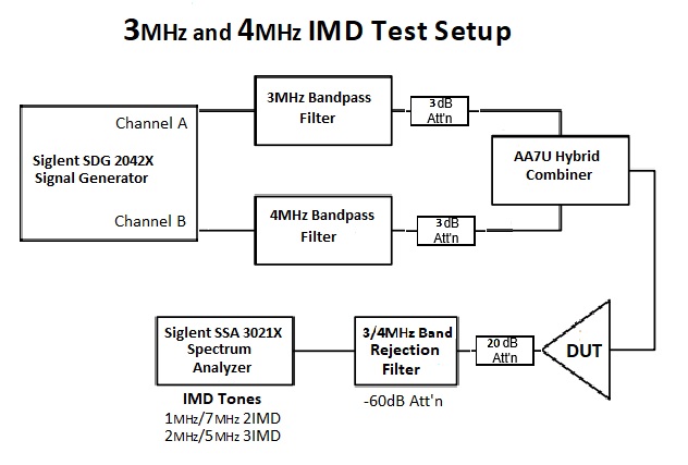
Siglent SDG2042X (AWG) Dual Channel Arbitrary Waveform Generator set up for use in IMD Test Set
- Turn on the AWG (arbitrary waveform generator) — wait for it to initialise.
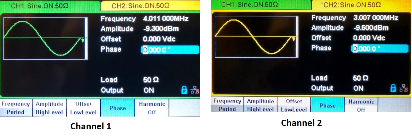
- Frequency is highlighted, with 1 kHz the default. Enter “3”, then touch “MHz” at the bottom left. (By touching the screen where it says Frequency, you can enter the frequency on the keypad “3” then at the bottom of the screen touch “MHz” and that will set the frequency).
- You will need to be set to 3 MHz (3.007 MHz) on Channel 1 and set 4 MHz (4.011 MHz) on channel 2 (Note: The reason for using the odd frequencies is the Siglent SSA3021X (SA.. or Spectrum Analyzer) has a sub-harmonic spur at 5 MHz)
- Load–HI Z is the default. Select “50 Ω” at the bottom, by touching the screen.
- Amplitude–2.00 Vpp is the default when in 50 ohms load. Enter “0”, then touch “dBm” on the bottom (fifth one over from the left–Vpp; mVpp; Vrms; mVrms; dBm). Make sure to set dBm.
- Output–OFF is the default. Touch it and it turns ON and the Ch1 indicator turns on with the button also, by its BNC connector.
- Repeat the above for Ch 2 as described above.
- Adjust Amplitude settings for each channel, which are going through the Band Pass Filter (BPF), 3 dB attenuator, combiner and DUT under test for a 0 dBm on the SA, with the SA internal Attenuator set at -20 dB.
(Note: As an example, this will be around (~ -10dBm). Make sure that the 3 MHz BPF is connected to the 3.004 MHz Channel and the 4 MHz BPF is connected to the 4.011 MHz Channel.
IMD Test Setup–Spectrum Analyzer setup for Siglent SSA 3021X
There are two parts to the setup–the first part sets the levels at the DUT output to 0 dBm; the second part measures the IMD.
Part 1
(Calibration) Push “Preset”, Top Right, to set up for initial setup.
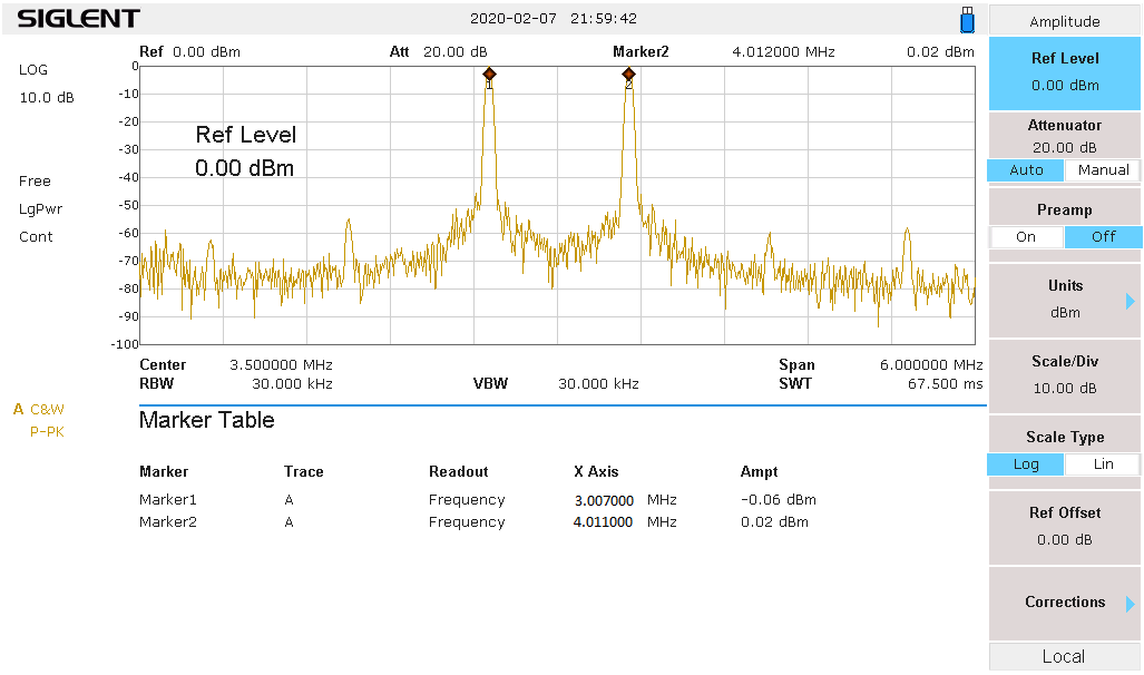
Set Center Freq 3.5 MHz, Span 6 MHz, Amplitude Ref Level +10 dBm
- Connect the DUT (Power On) output to SA input. Tune to one, either the 3 MHz, or 4 MHz test tones on the AWG. Adjust the generator (AWG) for 0 dBm on the SA, within 0.1 dB. Tune to the other test tone, adjust the generator for 0 dBm.
SA: Recheck each tone again to make sure nothing has changed. This concludes the initial setup.
Part 2
- Disconnect the DUT output from SA and connect it to the Reject Filter input (Which has the 20 dB built-in Attenuator). Connect the Reject Filter output to SA RF input.
2. Now look at the 4 IMD frequencies.
-
- Span set to 1 kHz
- Amplitude turn Preamp Off; set Ref Level to -60 dBm, Set Attenuation to Manual and set Attenuation to 0.00 dB.
- Push the Trace button and look for and select “Avg Times 100”, which is located on the right bottom side of the screen.
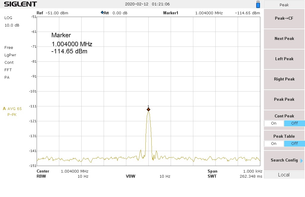
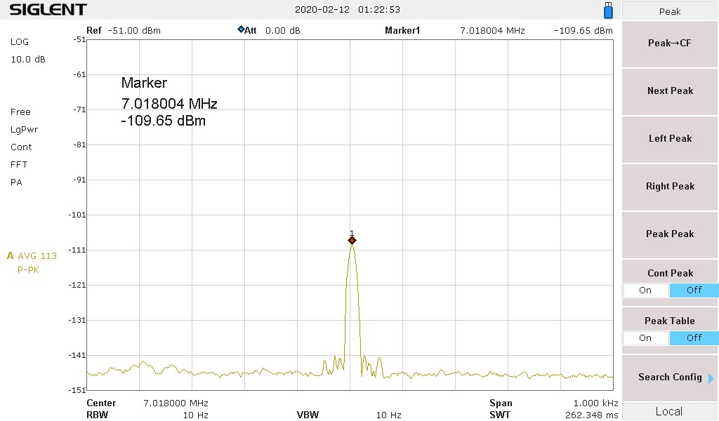
The 4 frequencies you will be looking at are: Center Freq 1 MHz (1.004 MHz), 7 MHz (7.018 MHz), 2 MHz (2.003 MHz) and 5 MHz (5.015 MHz),
- You should now be seeing the 2IMD product in the center of the display 1 MHz (1.004 MHz). Push the Peak button or push Marker button and use the main tuning knob to tune to the peak of the signal. It will probably vary up and down, but wait for 100 averages and decide what the middle value is and write that down.
- Tune to the 7 MHz (7.018 MHz) 2IMD product and note its level–write that down.
- Tune to 2 MHz (2.003 MHz) 3IMD product, this will normally be much weaker, where the SA’s preamp may be needed to see it. Write down that level.

- Tune to 5 MHz (5.015 MHz), write down that level. You now have measured the four IMD levels.

Use the formula for determining OIP2. (2IMD level – Reject Filter loss at that frequency 1 and 7 MHz) = OIP2.
Determine the OIP2 for both 2IMD frequencies. They are usually different–use the worst case, or specify both Output Intercepts.
Use the formula for OIP3. (3IMD level – Reject Filter loss at that frequency 2 MHz and 5 MHz) /2 = OIP3. Determine OIP3 for both 3IMD frequencies. Usually, they are about the same.
Examples
My reject filter has a -21.6 dB loss at 1 MHz; -20.39 dB loss at 7 MHz for the 2IMD frequencies. There is a -20.65 dB loss at 2 MHz and -22.62 dB loss at 5 MHz for the 3IMD frequencies.
The examples used in the below calculations were taken from the above IMD sweeps.
1 MHz (-109.65 dBm) – (-21.6 dB loss) = (109.65 – 21.6 = 88.5) = +88.05 dB OIP2.
7 MHz (-111.66 dBm) – (-20.39 dB loss) = (111.66 – 20.39 = 91.27) = +91.29 dB OIP2.
Normally you take the worst case and state that, which would be +88.05 dB
2 MHz (~-112.9 dBm) – (-20.65dB loss) = (112.9 – 20.65) = 92.25/2 = +46.13 dB OIP3.
5 MHz (~-111.66 dBm) – (-22.62 dB loss) = (111.66 – 22.62) = 89.04/2 = +44.52 dB OIP3.
Normally these should be very close, otherwise take the worst case, which would be +44.62 +dB
and state that.System IMD Intercept Test with Band Pass Filters, Combiner and 3 MHz and 4 MHZ Band Rejection Filter connected to the SA
They are all at the noise floor, which is very good. It took adding Band Pass Filters in place of Low Pass Filters to achieve the results Below.
1 MHz (1.004 MHz) -151.26 dBm
7 MHz (7.018 MHz -152.45 dBm
2 MHz (2.003 MHz) -153.51 dBm
5 MHz (5.015 MHz) -152.26 dBm
These are the simple formulas for second and third order IMD, you can take any two frequencies and work out the IMD products
Second order: F1 + F2; F2 – F1
Third Order: 2F1 + F2; 2F1 – F2; 2F2 + F1; 2F2 – F1
3 MHz and 4 MHz tones: 3 + 4 = 7 MHz ; 4 – 3 = 1 MHz; 6 + 4 = 10 MHz; 6 – 4 = 2 MHz; 8 + 3 = 11 MHz; 8 – 3 = 5 MHz
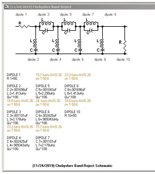
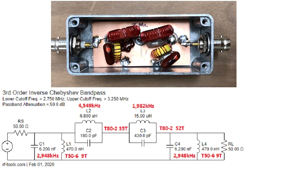
Building the Bandstop Rejection Filters
The easiest way to build and tune this filter is to test each Dipole (Tuned Circuit) by its self. It should be 3,250 kHz. Below is a sweep from my VNA, as this is what I used to check and tune each Dipole. I was able to tune the parallel circuits by having one side soldered to its pad and then connect the other end after tuning. You can also use the SIGLENT SSA3000X, SSA3000X Plus, or SVA to tune the filter.. as shown in this note on Filter Testing Using a SIGLENT Spectrum Analyser
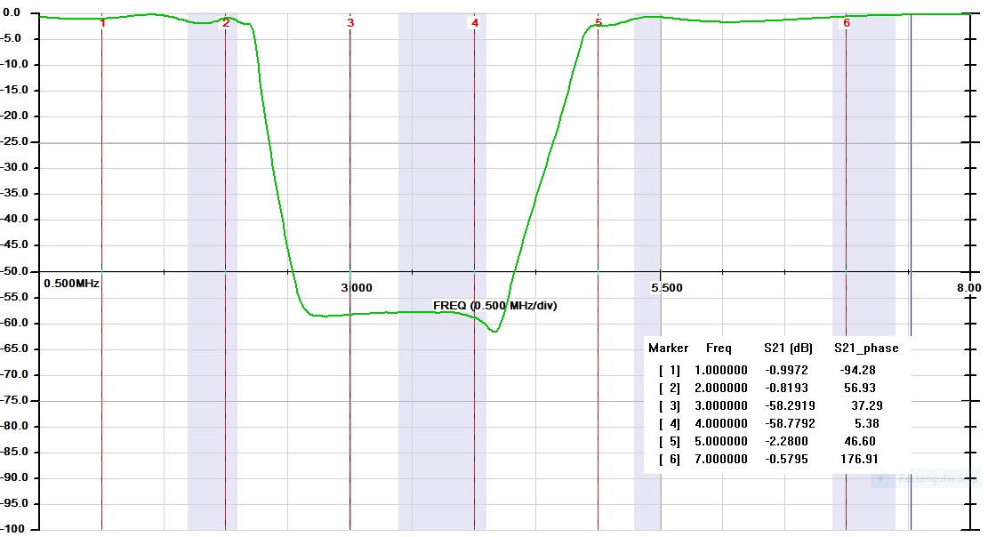
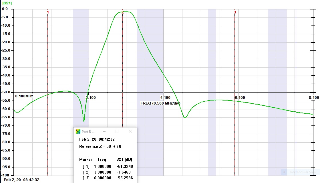
Below is a sweep of the final Band Rejection filter that is being used for IMD testing. There is around 58 dB rejection for 3 and 4 MHZ
Below is the finished 3/4 MHz Bandstop Filter and Sweep
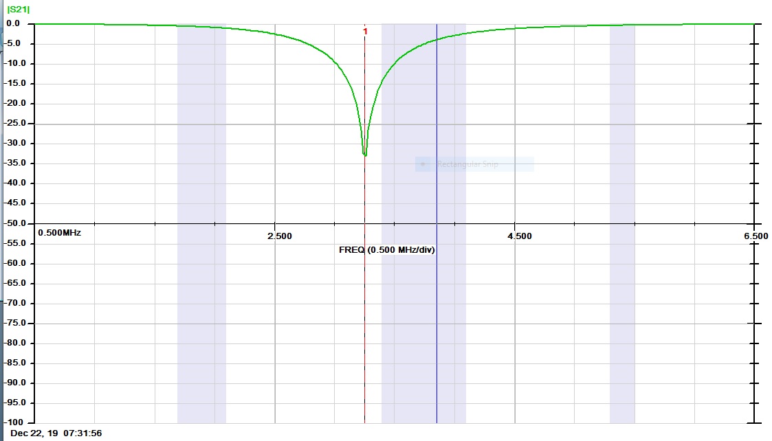
Below is a sweep of the final Band Rejection filter that is being used for IMD testing. There is around 58 dB rejection for 3 and 4 MHZ
A 20 dB pi pad can be done with 62 ohms shunts and a 270 ohm in parallel with 3300 ohms for the series resistor. (249.6 shown on the diagram. The theoretical value is 248 ohms.)
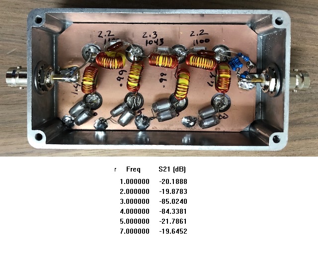
Both the 3 MHz and 4 MHz Bandpass filters are easy to build if you will tune each pole and install it as you go. I have marked the frequencies in Red for each pole. Also, I have indicated which Micrometal Toroids that were used with the turns required for each pole. You may have to make some adjustments to each of the poles, as there are variations from lot to lot with the toroid core. I also found it helpful to use an LCR meter to make adjustments in the turns count to get the desired inductance. I used an Array Solutions VNA2180 to tune each pole and evaluate the final filter. A SIGLENT SVA1000X VNA can also be used.
4 MHz BPF
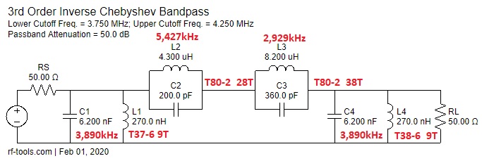
3 MHz BPF
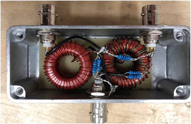
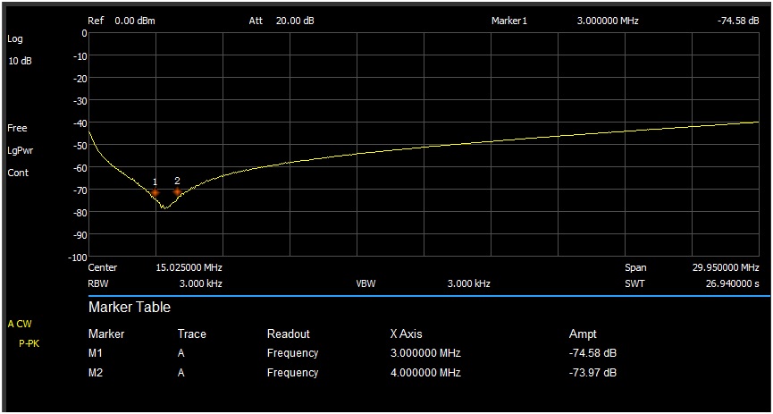
AA7U Hybrid Combiner
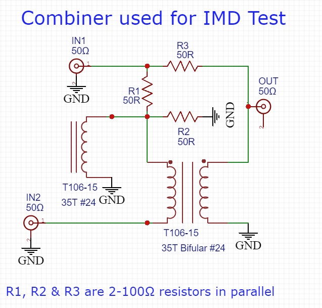
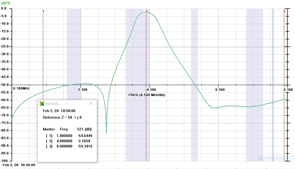
The loss through the filter is 6.13 dB/5.95 dB and the isolation between the two input ports is 74.58 dB at 3 MHz and 73.97 dB at 4 MHz (Measured with a 50Ω Termination at the output port.) After completing and testing the filter I filled it up with hot melt glue.
Below is a sweep of the Hybrid Combiner between the two input ports and it was terminated with 50Ω at the output port.
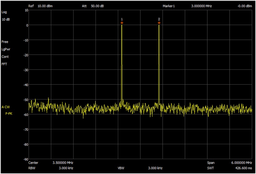
This is a sweep showing the two test tones 3 MHz and 4 MHz using the Hybrid Combiner. Notice how sharp they are.
How to take screenshots of the Siglent SA
Insert the thumb drive into the front USB port of Siglent.
You should see a blue USB icon in the upper right-hand corner of the screen.Hit the File button
You should see a file directory similar to what you would see on a PC.Under the Folder column, you should see two directories:
Local: free 80.74 MB (your size may be different)
+U-disk0: 748.00 KB/975.88 ME (your size may be different)On the right-hand side soft keys, the “Save Type” should be PNG.
Hit the button and select JPG (or whatever file type you want – CSV, LIM, JPG, BMP, etc.)Rotate your frequency tune knob and select your +U-disk0 directory
You should see the files currently on your thumb driveHit the Enter button
Hit the Operate button
Hit the Marker button
You should now be back at your main display screenSetup a screen that you want to save
Hit the Save button
A pop-up window will show you a default file name of Name: JPG1 and an Input type: abc
I like to use a numeric file name, so I hit the +/- button
Now I backspace out the default “JPG1” file name
I enter the numeric name that I want to use. Example: 111
I find it quicker to use quick numeric file names and rename the file once the thumb drive is attached to my PCHit the Enter button
You may or may not see a brief text message on the screen about the screen being saved to your thumb drive.To confirm that the file was saved to your thumb drive, Hit the File button
Use the Frequency control knob and select your thumb drive directory
In the directory listing for the thumb drive, you should see your recently saved screen snapshotFor some reason, the screen sometimes saves to the internal Siglent memory. When this happens, I go through the steps again about setting up a save to the thumb drive. I suspect that my steps are a little flakey in this area.
Once the Flash drive is set up you can save the screenshots by pressing the Save button, which will number the shot and then press the Enter button.
Products Mentioned In This Article:
- SDG2000X Series please see HERE
- SSA3000X Series please see HERE
- SSA3000X Plus Series please see HERE
- SVA1000X Series please see HERE
Multi Channel function generator synchronisation
1. Introduction
Multi-channel function generators are useful in many situations. For example, in Radar testing the generator needs to output several phase coherent signals and for the phase to be independently adjustable for each signal. In 3-phase power line harmonic distortion testing, a 4 channel generator is required to simulate the multiple voltages and currents.
1.1 Problem
A standalone multi-channel generator can be very expensive.
1.2 Solution
Siglent provides the Multi-Device Synchronisation function in the SDG1000X, SDG2000X, and SDG6000X generators. This allows synchronization among several units in order to output signals with adjustable steady phase relationships. Thus saving on cost.
2. Setup of Synchronisation
2.1 Wiring
Multi-Device Synchronisation will require the use of the Aux In/Out and 10 MHz In/Out rear-panel interfaces to implement the synchronisation. First, all the generators’ Aux In/Out BNC connectors need to be connected together. Next, connect the Master unit’s 10 MHz Out to the Slave unit’s 10 MHz In. Please note that the SDG6000X family has separate 10 MHz In/Out outputs, so more than two units can be synchronized. The wiring interconnection concept is shown in Figure 1.
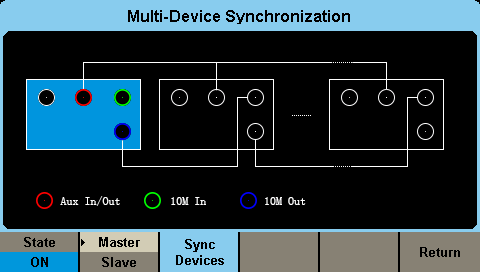
Figure 1. Wiring concept
However, the SDG2000X and SDG1000X series’ 10 MHz In/Out ports share one connector. Therefore, only two units can be synchronized together or they must be the last Slave unit in a multiple units connection.
In this note, the SDG2000X and SDG6000X series models are used as our example. The SDG6000X will be the Master device.
1) First connect two units’ Aux In/Out with BNC cable. See in Figure 2.
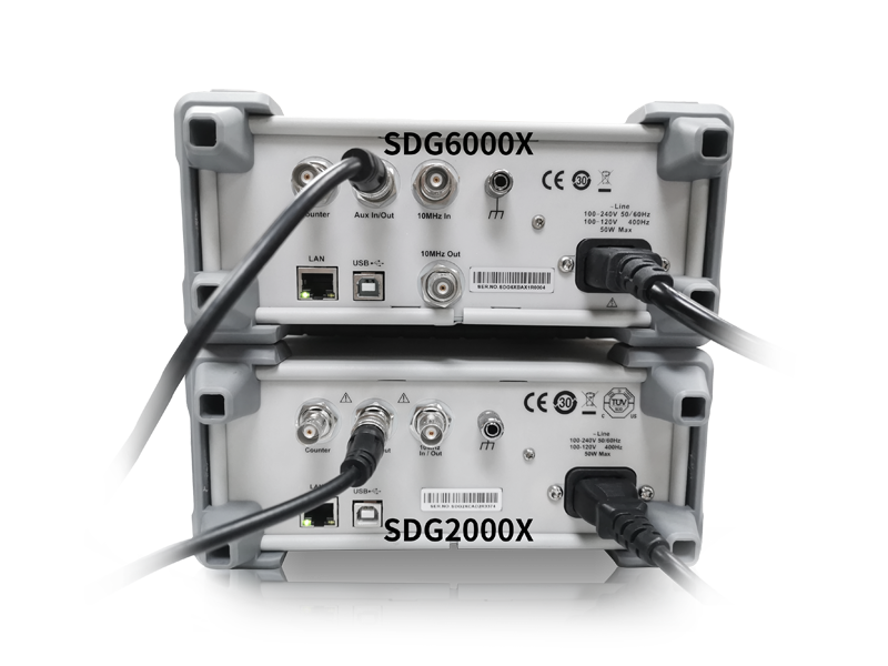
Figure 2. Connect SDG2000X and SDG6000X Aux In/Out
2) Next connect the SDG6000X 10 MHz Out port with the SDG2000X 10 MHz In/Out port, as shown in Figure 3.
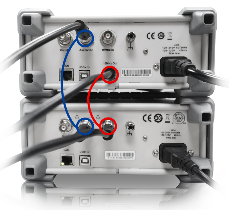
Figure 3. Connect Master 10 MHz Out to Slave 10 MHz In
2.2 Parameter settings
Set the waveform parameters, such as Frequency and Amplitude, on 4 all channels. More information on this step can found in the User Manual.
Press Utility, go to Page 2/3, choose Phase Mode, and then set both units as Phase Locked.
In this example we are setting all 4 channels as a 1 kHz, 4 Vpp square wave. CH3, CH4 signals viewed on the SDS5000X oscilloscope are output by the Slave generator, note that the phase is drifting. Open the Display/ Persist function to track it on the scope, as shown in Figure 4.
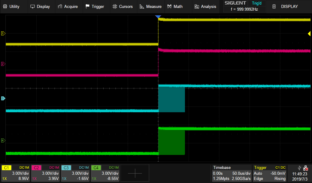
Figure 4. Four signals phase drift without synchronisation
2.2.1 Set Master Device
1) Press Utility button, go to Page 3/3, then press the soft key under screen to select Multi-Device Sync. The menu will enter the Multi-Device Synchronization screen, shown in Figure 5.
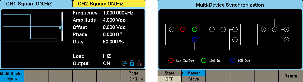
Figure 5. Multi-Device Synchronisation Screen
2) Press the soft key under the screen to turn on/off this function and select it as either the Master or Slave. The Multi-Devices Synchronisation menu will appear when turned on. When ”Master” appears shaded in light gray this means the device is designated as the Master device, as shown in Figure 6. When this device is set to be the master, its clock source is automatically set to internal and the 10 MHz output is enabled.

Figure 6. Turn on synchronisation function
2.2.2 Set Slave Device
1) Enter into the Multi-Device Synchronisation menu. Select it as Slave, Slave will be shaded in blue, as in Figure 7. As the device is set to a slave device its clock source is automatically set to external.
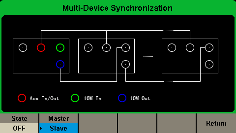
Figure 7. Select the unit as Slave device
2) Turn on the State. Then the Slave Device Delay window will occur. Press to enter delay value, as shown in Figure 8.
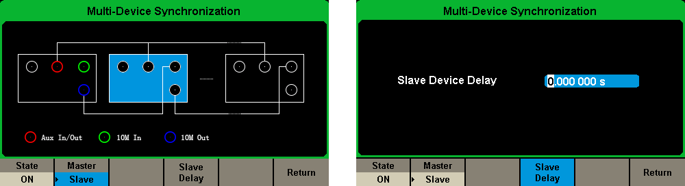
Figure 8. Set the Slave Delay
2.2.3 Synchronise the Devices
Press the soft key ”Syncs Devices” in the Multi-Device Synchronisation interface of the Master device, as shown in Figure 1, to begin synchronisation between the master and slave devices. Anytime a setting is changed; for example, the Slave Device Delay, ”Sync Devices” must be pressed to activate the new settings.
3. Measure on an Oscilloscope
3.1 Slave Device Delay measurement
1) Turn on Synchronisation on both units, measure the Skew between CH1 and CH3. As in Figure 9.
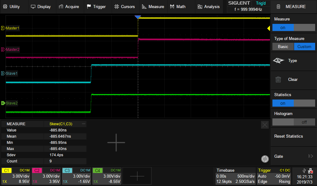
Figure 9. Measure the Skew between Master and Slave Devices
2) Enter the absolute Mean value of Skew into Slave Device Delay. This will eliminate the delay between traces that we observed with our oscilloscope. See Figure 10.
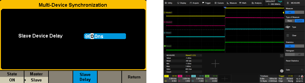
Figure 10. Eliminate the Slave Delay
3.2 Adjust phase relationship
Set CH1 Phase as 0 degree, CH2, CH3, CH4 Phase as 180, 270, 360 degrees, respectively. The result is shown in Figure 11.
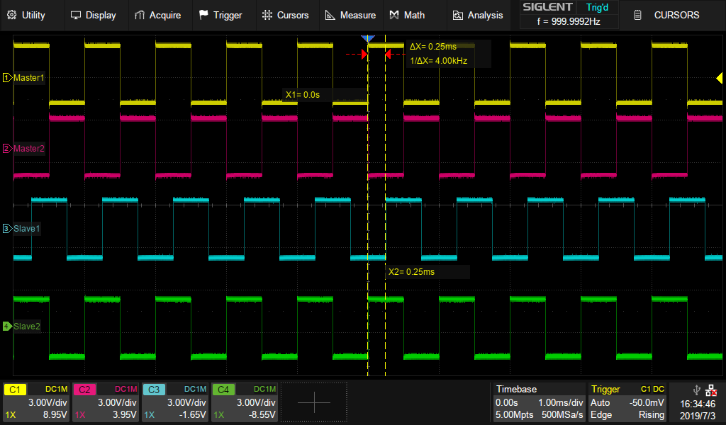
Figure 11. Adjust phase relationship
Products Mentioned In This Article:
Secure products without K-lock slots
Many products have Kensington, or K-lock slots to help provide a location to secure a cable lock or other device to help prevent theft.
Some products do not have locations for cable lock connections.
In this case, we recommend using a special glue or physical attachment system to secure the cable to the case of the instrument.
Here is an example:
https://www.kensington.com/p/products/security/lock-anchor-points-accessories/security-slot-adapter-kit-for-ultrabook/
AWG Basics
Many electronic designs feature the ability to monitor or measure input signals and then perform another task or function based on that input signal. A simple example could be a circuit that looks for an input voltage to exceed a specific amount and triggers another action after it occurs. In such cases, having the ability to configure and deliver a known or simulated signal can be a critical addition to testing the performance of the design. Unlike acquisition instruments that measure a signal, an input signal can be created using a signal source. This can be as simple as a DC power supply or as complex as a digital communication signal delivered by an RF Vector Source. One of the most flexible and useful signal sources available today is the Arbitrary Waveform Generator (AWG).
In this series of notes, we are going to introduce some of the features that make AWGs so useful and explain in a bit more detail just how they work.
What types of signal sources are on the market today?
Let’s start with the basics. Most sources can be divided into two broad application categories: Digital and Analogue.
Signal sources specially created for digital applications are often called logic sources. Logic sources can be roughly divided into two categories: Pulse and pattern generators. A pulse generator can output square waves and pulse streams. The output frequency of the pulse generator is generally very high and it is often used to test digital devices. A pattern generator, also known as a logic source or data generator is a bit unique. This kind of instrument generally has 8 or 16 output channels, but higher channel counts are available. Each output can generate various types of synchronous digital pulse streams, generally from a low to a high voltage value, 0-5 V for example. Pattern generators are often used as excitation signals for computer buses, digital telecommunications units, and other serial communications links.
Analog generators typically have one or two outputs and feature a wider array of possible output levels, wave shapes, and frequencies than digital sources. More specialised forms of analogue generators also exist for high frequency applications. We aren’t going in to further detail about them here, but some common types include RF signal generators, microwave signal generators, and baseband signal generators.
In this article, we will concentrate on the most general purpose signal source, the arbitrary waveform generator. In simple terms, an arbitrary waveform generator is a device that creates an output signal based on a digital waveform file, created from a series of discrete output sample points, and “plays” the file contents at the source output of the generator. Using this sampling principle, waveforms of almost any type can be created, including basic waveform functions like square, sine, and ramping output shapes.
Arbitrary waveform generators can also have more advanced functions like output triggering and system clock signals for synchronizing external instruments. One such generator is the SIGLENT SDG2000X series function / arbitrary waveform generator shown in Figure 1 below.
Figure 1: SIGLENT SDG2000X function / arbitrary waveform generator
What is the waveform generator used for?
As mentioned previously, most arbitrary waveform generators include basic function types like sine, square, and triangle waves. In addition, waveform generators can also generate analogue and digital modulation signals, supporting the output of linear / logarithmic sweep signals and pulse trains. Many of SIGLENTs SDG series of generators support AM, FM, PM, FSK, ASK, DSB-AM and other analogue and digital modulation functions and include a large standard library of included arbitrary waveform functions.
There are hundreds of applications for waveform generators, but in the field of electronic test and measurement, the application range can be basically divided into three types: inspection, verification, and limit / margin test. During the commissioning phase of a design, the engineer needs to test the parameters of the product to verify whether the product meets the relevant design specifications. In this process, the waveform generator can be used to source the signal specified in the design specification. Here, the Engineer can observe the response of the design, compare the results with the specifications, and perform any adjustments that may be necessary with the design. In addition, newly developed industrial control modules, data conditioning modules, and others all need to use waveform generators to test their linearity and monotonicity through exhaustive testing. In many occasions, the waveform source needs to add a known, repeatable distortion in quantity and type to the signal it provides. With many generators, you can add noise and programmed distortion to the signal and directly test the ability of the design to handle specific real-world signal issues.
What are the main indicators of the waveform generator? What do these indicators mean?
Oscilloscopes have common banner specifications: Bandwidth, memory depth, and sampling rate. When we select a suitable oscilloscope, these three major indicators are often our first consideration.
Does the waveform generator also have the so-called three major indicators? The answer is yes. In the category of waveform generators, there are also concepts of bandwidth, sampling rate and memory depth.
- Bandwidth
The bandwidth of the waveform generator is often defined as the maximum frequency of a sine wave. Unfortunately, what applies for a sine wave may not apply to other waveform types. For example, the maximum sine wave output frequency of the SIGLENT SDG2122X is 120 MHz, while the square wave has a maximum frequency of 25 MHz. The reason for this difference is that a square waveform transitions very quickly from one voltage value to another. Faster transitions require that the waveform contains many higher-frequency components than the smooth transitioning sine wave. In order to avoid heavy distortion of the rising edge of the square wave output, when the waveform generator outputs a square wave, its bandwidth range must be able to include these higher harmonic components.
- Sampling rate
The sampling rate of the waveform generator is usually expressed in mega-samples (MSa/s) or giga-samples per second (GSa/s). For example, the nominal sampling rate of SDG2000X series function / arbitrary waveform generator is 1.2 GSa / s. This parameter indicates the output rate of each sample of the waveform being sourced. The Nyquist sampling theorem stipulates that the sampling rate or clock rate must be at least twice the highest spectral component of the generated signal, thus, accurate reproduction of the original signal can be guaranteed. But in practical applications, twice is often not enough, depending on the type of signal and the rise time. Higher output sampling rates indicate that a signal source is capable of sourcing samples quickly. Low sample rates can limit a generators ability to accurately source a given waveform type.
Here is a quick example.
If you have a waveform made of 1,000 samples and your generator can source 10 MSa/s, the maximum output frequency of the waveform can be calculated as follows:
Frequency = Sample Rate/Samples = 10 MSa/s / 1000 Samples = 10 kHz.
So, the sample rate and number of samples used to create your waveform determine the output waveform period and can be a quick test to determine if the generator will work for your application.
- Memory depth
Memory depth refers to the number of data points used to record the waveform, which determines the maximum number of samples of the waveform data. The bandwidth of the waveform generator is determined by the sampling rate and memory depth. The SDG2000X series function / arbitrary waveform generator supports “point-by-point output”, which can output 8 pts ~ 8 Mpts at a variable sampling rate of 1 uSa / s ~ 75 MSa / s without losing waveform details. Deeper memory provides higher resolution in the time domain and enables users to create more detailed waveforms.
In addition to the above three indicators, frequency resolution and vertical resolution are also important indicators of waveform generators. Vertical resolution refers to the smallest voltage increment that can be programmed in the waveform generator, and is related to the number of DAC bits used in the hardware circuit. It is generally expressed in units of “bits”, which determines the amplitude accuracy of the output waveform. Frequency resolution, the smallest adjustable frequency resolution, that is, the smallest time increment that can be used when creating a waveform, is related to the highest rate of the clock and the conversion rate of the DAC.
The waveform generator is one of the most widely used basic general-purpose instruments and it is an indispensable tool for simulating signals and testing your design performance. For more information, search out our additional articles to give you more understanding of the principles of the waveform generator.
Products Mentioned In This Article:
SDG2000X Series please see HERE
The basic output waveform and related parameters of the arbitrary waveform generator
Traditional function generators can output standard waveforms such as sine waves, square waves, and triangle waves. However, in actual test scenarios, in order to simulate the complex conditions of the product in actual use, it is often necessary to artificially create some “irregular” waveforms or add some specific distortion to a waveform. Traditional function generators can no longer meet the requirements and an arbitrary waveform generator may be a good option.
Arbitrary waveform generators can easily replace the function generators. They can source sine waves, square waves, and triangle waves like a standard function generator. In addition, they can also output pulse, noise, DC signal types, modulated signals, sweeps and bursts. Many arbitrary waveform generators currently on the market are equipped with arbitrary waveform drawing software. Through this software, theoretically, the arbitrary waveform generator can be remotely controlled to output all the signals required in the test process.
So, what types of waveforms can an arbitrary waveform generator output?
What parameters are available for an arbitrary waveform?
How to measure the quality of the output waveform?
- Sine Wave / Cosine Wave
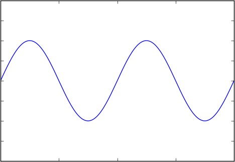
Figure 1 Sine wave / Cosine wave
Sinusoidal (sine) and cosine waves are the two most familiar waveforms in electronics.
Sine/cosine waves are defined as follows.
 (Formula 1)
OR
 (Formula 2)
Where A represents the amplitude of the sine wave,
 represents the angular frequency, and
  represents the initial phase, which can be omitted in the general calculation. The sine and the cosine waves are essentially the same, but the initial phase differs by 90 °.
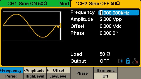
Figure 2 Sine wave setting interface in SDG1000X
These three parameters are as shown in Figure 2. The frequency and period related to the angular frequency can be set in the arbitrary waveform generator, and the conversion relationship between them is:
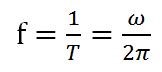 (Formula 3)
The frequency of a generator, like the SIGLENT SDG2122X function / arbitrary waveform generator sine wave can be set up to 120 MHz. Usually, the nominal maximum output frequency of the arbitrary waveform generator often refers to the maximum frequency of its sine wave output.
You can also set the amplitude, A. When the output impedance is set to the “high impedance” state, the maximum output amplitude of the SDG2122X can reach 20 Vpp.
The initial phase can be set by clicking the corresponding button in the [Phase] menu. The range of the initial phase can be set between -360 ° and + 360 °.
From the time domain perspective, the parameters and waveforms of the sine and cosine waves are relatively simple. However, all electronic devices have more or less distortion, and arbitrary waveform generators are no exception. Let’s observe sine and cosine waves in the frequency domain.
The Fourier transform corresponding to the time domain function represented by Formula 1 is:
 (Formula 4)
The spectrum diagram represented by Formula 4 is shown in the figure below:

Figure 3: Cosine spectrum/frequency domain
Looking at the cosine spectrogram (showing amplitude vs. frequency) in Figure 3, we can find that the frequency of a sine/cosine wave can be represented by a single line on the spectrum. Signals that occupy only one frequency are called “monotone” because they only have one frequency component.
In engineering, due to the non-ideal characteristics such as the non-linearity of the circuit, the generated sine wave is often not an ideal monotone signal, but may contain other frequencies. Collective “unwanted” frequencies are often lumped together under the term distortion. Some common contributors to distortion are harmonics and spurs.
- Harmonic distortion
The fundamental frequency of a signal is the lowest frequency component of a periodic signal. Harmonics are the frequency components of the signal that are integer multiples of the fundamental. Distortion is the ratio of signal power to maximum harmonic power, usually in dB, as shown in the following figure:

Figure 4: Harmonic distortion
Another index to measure the performance of harmonic distortion is total harmonic distortion (THD), which refers to the ratio of the root mean square of the amplitude of each harmonic (usually taken to the 6th harmonic in engineering) to the signal amplitude, as shown in Formula 5, usually expressed in %. When an SDG2000X outputs 0 dBm, 10 Hz ~ 20 kHz sine wave, the total harmonic distortion is 0.075% at most.
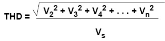 (Formula 5)
- Non-harmonic spurs
In addition to harmonics, the distortion caused by nonlinearity may also be some other spectral components, such as the intermodulation products of the signal (or its harmonics) and the clock signal. It is necessary to define other index-non-harmonic spurs to measure.
The size of the spur is usually expressed by the spurious-free dynamic range (SFDR) (see Figure 5), which refers to the ratio of the signal power to the maximum spurious power. The unit is usually dB. Please note that the definition of spurs in some places includes harmonic and non-harmonic spurs, but in arbitrary waveform generators, spurs only refer to distortions other than harmonics.
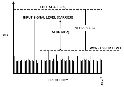
Figure 5: SFDR
Products Mentioned In This Article:
Generating an Activation Code (Option Code)
Introduction
Many SIGLENT products have options that can be activated by entering a special activation code into the front panel.
This note covers how to generate the activation code.
Setup
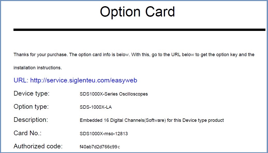
- Contact your Authorised SIGLENT sales office or distributor to obtain an Option Card. This is typically a document that is emailed as a PDF.
A typical Option Card will contain the following information:
This is the official SIGLENT website for generating activation codes.
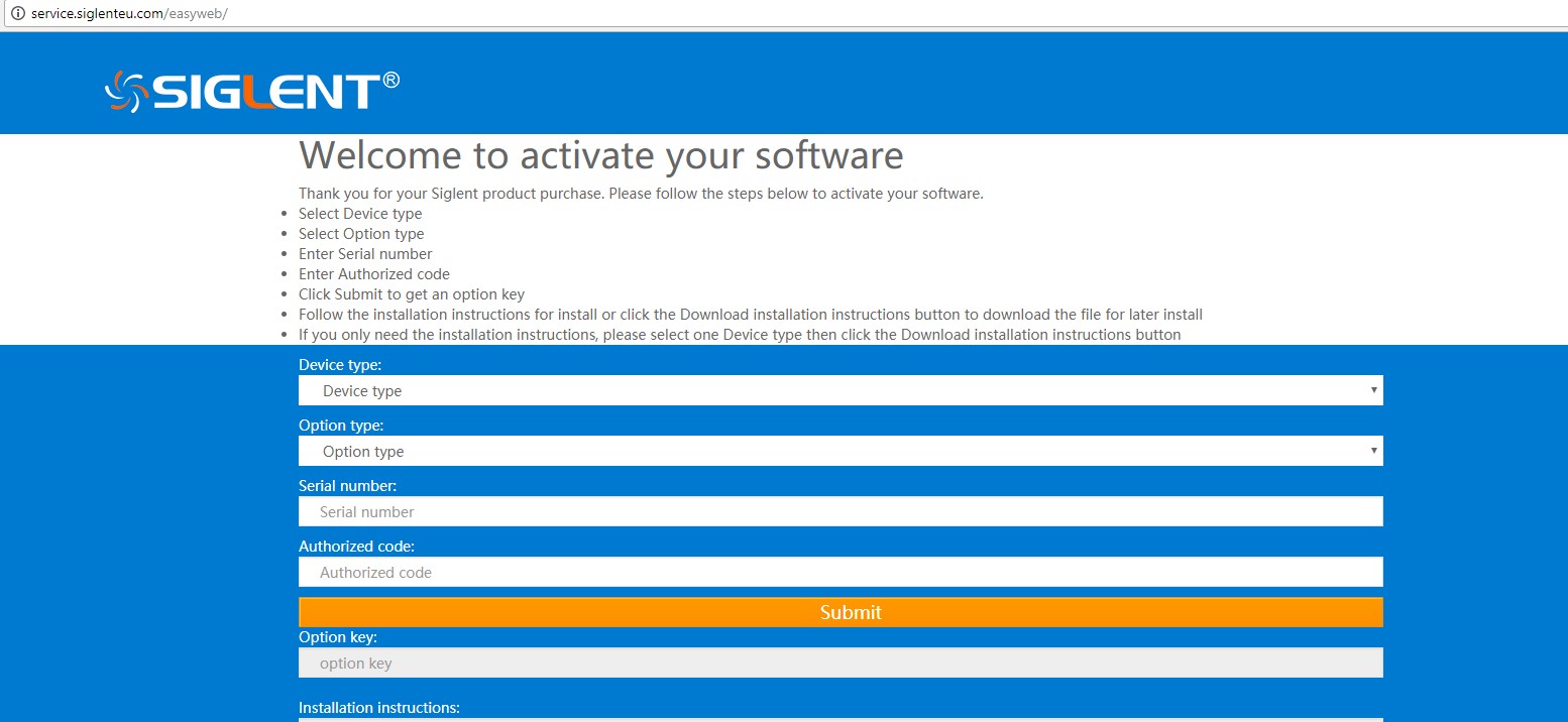
- Select the Device Type (Product Model Family)
- Select the Option Type (The option card you purchased)
- Enter the Serial Number of the instrument you wish to add the option to
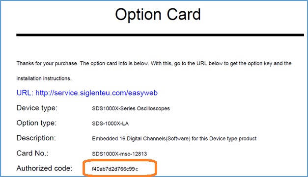
- Enter the Authorisation Code from the Option Card (example circled below).
- Press Submit. This will generate the Option Key which can be entered into the instrument and permanently activate the option.

NOTE: See the specific instrument user’s manual for instructions on entering option codes
EasyPulse Technology and Its Benefits
INTRODUCTION:
The majority of modern arbitrary/function waveform generators utilise DDS technology (Direct Digital Synthesis), but there are a few obvious defects using this technology directly. To solve these disadvantages, SIGLENT invented a pulse generating algorithm called EasyPulse technology. In this note, we will describe the basics of DDS and how EasyPulse can help get the best performance possible.
1.DDS technology and its disadvantages
Direct digital synthesis (DDS) is a technique to produce an analogue waveform (square, triangular, or sinusoidal) by generating a digital time-varying signal in digital form and then performing a digital-to-analogue conversion. A basic Direct Digital Synthesizer consists of a frequency reference (often a crystal or oscillator), a numerically controlled oscillator (NCO) and a digital-to-analogue converter (DAC), the block diagram is shown in Figure 1.
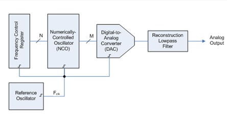
Figure 1: Block diagram of DDS circuit The reference clock is a fixed frequency (Fref). DDS generates the waveform by looking up the pre-loaded 2N data samples from memory.
The Tuning word (M) stored in the register determines the frequency of the output:
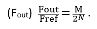
Since the edges of square/pulse signals output through the DDS technology are fixed, and the duty-cycle is limited by the data length, there will be poor duty-cycle setpoint resolution at higher output frequencies.
When generating a square/pulse, the reference frequency should be an exact integral multiple of the output frequency. If it is not an exact integral multiple, it will introduce a deterministic jitter equal to one reference clock period.
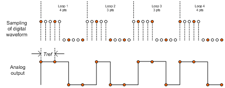
Figure 2 When the Tuning word >1 (i.e. Fout >Fref /2N ), some points in the sample lookup table are skipped. This is generally not a big problem for sinusoidal waveforms, but for arbitrary waveforms with some important details (e.g. spikes), it may mean the loss of information.
2.EasyPulse technology and its benefits
To solve these problems, Siglent invented a pulse generating algorithm called EasyPulse, which is applied to all of the SDG X series waveform generators.
Based on this new technology, the SDG series waveform generator is capable of generating a pulse signal with low jitter, rapid rising and falling edge (independent from frequency), small duty cycle( pulse width), edge and pulse width can be adjusted in a wide range. Figure 3 is the block diagram of EasyPulse:
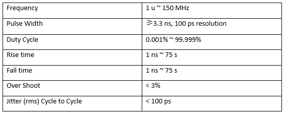
Figure 3: Block diagram of EasyPulse Take the SDG6052X series Pulse/Arbitrary Waveform Generator as an example, its specification for a pulse signal are as follows:
 3.Measurement examples
Equipped with the EasyPulse technology, the SDS6052X series Pulse/Arbitrary Waveform Generator delivers great performance. Let’s take a look at some real-world examples:
First and foremost, the EasyPulse technology could overcomes the additional jitter in Square/Pulse waveform generated by traditional DDS. To evaluate this excellent feature, we compared a DDS waveform generator with the SDG6052X with EasyPulse. In figure 4, we used a 12-bit scope to observe the differences. When the Pulse is trigged, measuring the next rise edge, we observe a 0.84 ns (which is equal to the period of the DDS clock, 1.2 GHz) peak-peak jitter if the pulse is generated by traditional DDS, while the jitter downs to 11.2 ps rms when we choose EasyPulse technology to generate the pulse with same configuration.
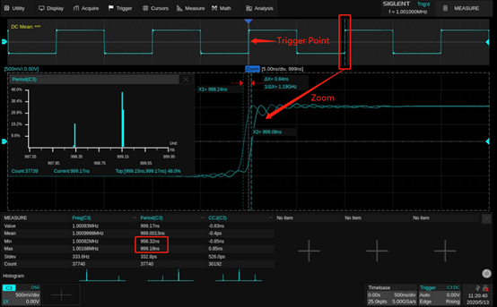
Figure 4: Jitter from a traditional DDS waveform 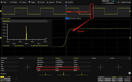
Figure 5: EasyPulse waveform with low jitter Another advantage of the EasyPulse technology is its ability to output the pulse with a small pulse width around 3.3 ns, even at very low frequency. For a 1 Hz pulse generated by DDS technology, there are 32768 points in one waveform length. If we built the pulse with only one sample point at the high level, we could get a pulse with the minimum pulse width (minimum duty ratio as well), which is about 30 ms (1 s/32768 ≈ 30.5 ms), as shown in figure 6. With EasyPulse, the width can be adjusted down to 3.3 ns as shown in figure 7.
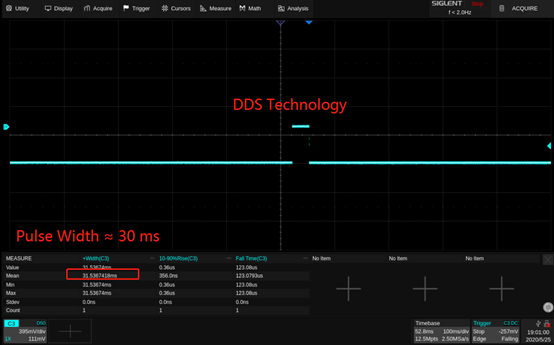
Figure 6: 1 Hz pulse signal generated by DDS 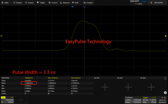
Figure 7: 1 Hz pulse signal generated by EasyPulse In addition, with the EasyPulse technology, both the edge and pulse width can be adjusted over a wide range. The pulse width can be fine-tuned to the minimum of 3.3 ns with an adjustment step as small as 100 ps, at any frequency. In figures 8 and 9, we used a 12-bit scope with infinite persistence to show the rising edge changes with pulse width settings from 3.4 ns to 200 ns with 100 ps each step.
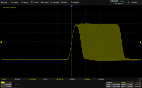
Figure 8: Adjusting the pulse width with 100 ps each step The rise/fall times can also be set independently to the minimum of 1 ns at any frequency with a minimum adjustment step as small as 100 ps. Output an initial pulse by the SDG6052X as the following parameters:
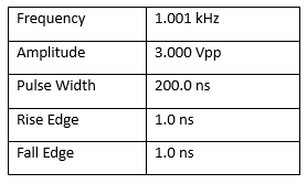
Figure 9 shows the rising edges of the SDG6052X Pulse/Arbitrary Waveform Generators from 1.0 ns to 100.0 ns step by step with 100 ps.
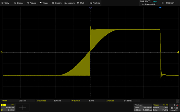
Figure 9: adjusting the rise time with 100 ps each step In conclusion, EasyPulse technology enables SIGLENT Pulse/Arbitrary Waveform Generators to perform excellently when generating a pulse signal with low jitter, small duty cycle, precise and adjustable pulse width.
Products Mentioned In This Article:
Analysing GSM Radio Protocol with a Siglent SDS2000X Plus Oscilloscope
We took a retired Siemens A36 cellphone to learn the capabilities of this new Siglent scope. Available documentation and medium-density PCB of the selected A36 made the signal probing easy to implement. We used TEK P6243 active probes initially for their low capacity loading but changed to passive probes later as monitored signals proved to be quite robust.
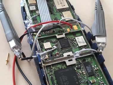 Figure 1: probing IQ signals in Tx and Rx path of the Siemens A36
Three signals were selected to monitor the cellphone operation:
- Transmit IQ baseband modulation signal, Q component, on Pin 48 on scope Channel 1
- Receive IQ baseband modulation signal, I component, on Pin 12 on scope Channel 2
- Battery current consumption from 0.1 Ohm resistor, between (-) power supply and phone ground on scope Channel 4 (resulting in negative signal polarity)
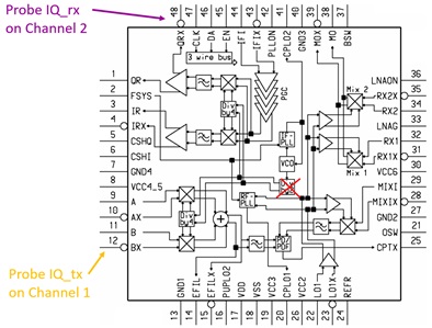
Figure 2: block diagram of PMB6250 Smarti IC with probe inputs
At first we observed the phone attached to the GSM network, periodically listening for an eventual incoming call on paging channel once per second. Once every 33 seconds, the phone is additionally checking the signal level of other base stations to request the network to camp on the stronger base station in the case when the phone is moving.
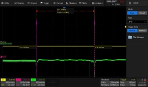
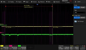
Figure 3: Rx signals for paging (left) and neighbour cell measurements (right)
Current peaks of 30 mA at the end of Rx signal burst indicate the processing power needed for decoding of the received signal. Neighbour channel measurement need only a part of the burst, allowing for frequency switching (PLL re-tuning) between the 3 bursts. We can see how noisy the other base stations are, and that the first burst of the serving base station has the least noise of all.
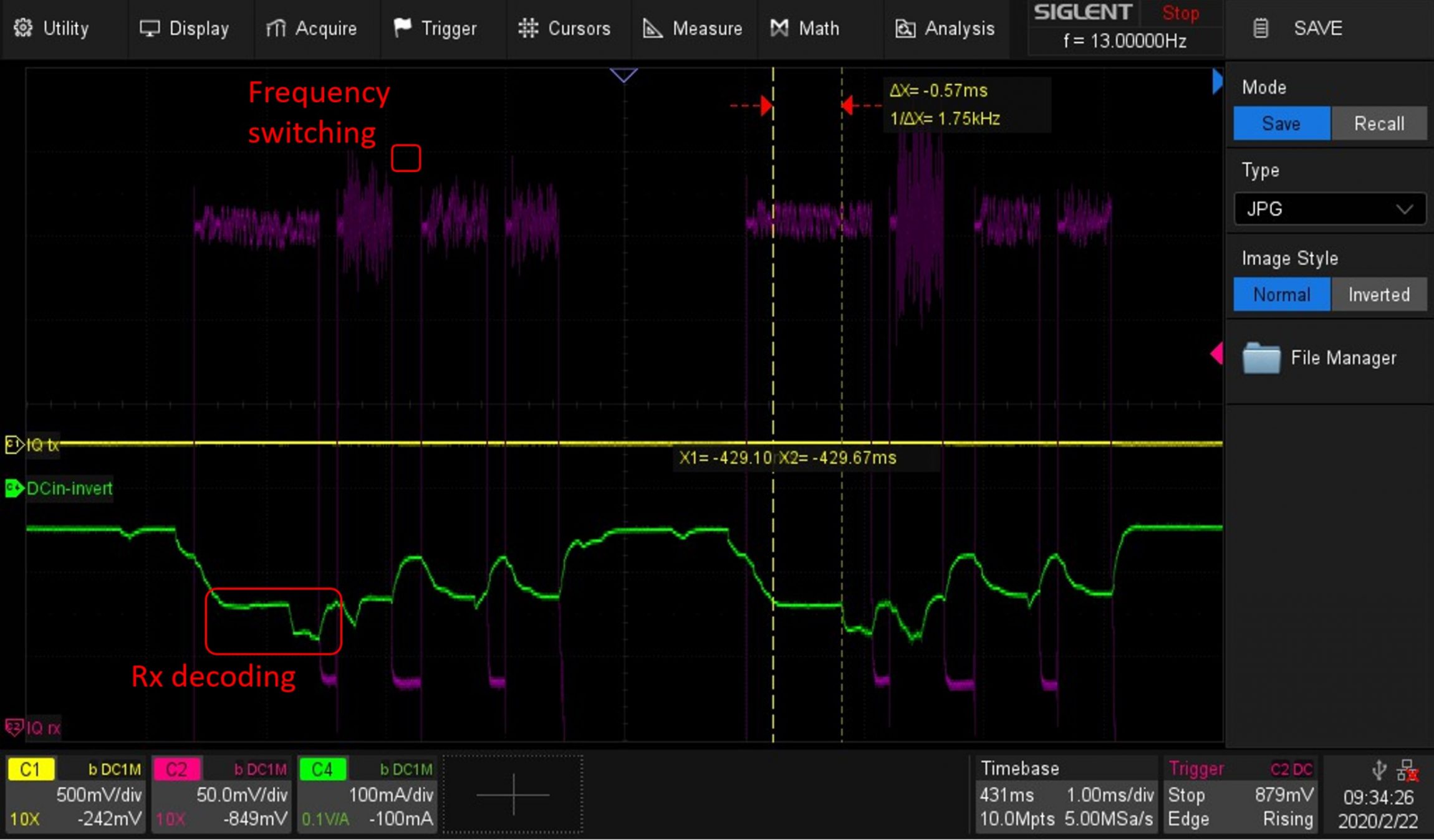
Figure 4: Rx signal detail and processing power (power consumption)
Using the scope persistence and colour histogram, we can visualise the received signal. We also used the scope Zone Trigger function (area 1) to distinguish between the longer data and shorter paging channels. We see the signal reception is longer than the data burst length of 570 µs. This allows for the demodulation of signals that may be dealing with multipath propagation. In a mountainous region, for example, base station signals can reach the phone on the direct fast track but may also propagate along a path with multiple reflections. Up to +-3 symbols delay can be processed by the A36 channel equaliser.
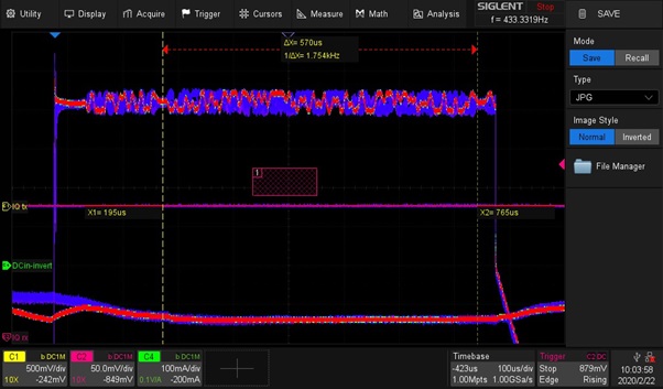
Figure 5: Histogram of Rx signal with 1 sec persistence
Then we set up a call between the phone and the network. For the first time, we can see the phone transmitter operation (yellow Channel 1). As the phone receives an incoming call from the paging channel it changes from idle to the call state after the user picks up the call of the ringing phone.
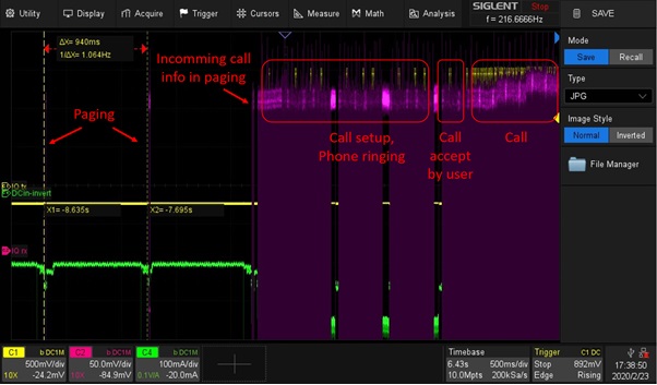
Figure 6: Incoming call setup flow
Parallel to the call, the phone still performs neighbour cell measurements for the case it finds a stronger base station that can handover the call.
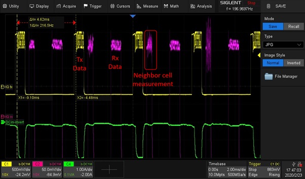
Figure 7: Call Tx and Rx bursts
On the transmit burst we can observe the permanently changing data bits carrying the speech signal. The static non-changing bits are the Tail Bits at the beginning and the end of the burst. Most important is the Training Sequence in the middle of the burst. The channel equaliser of the receiver is training its best adjustments on this training sequence and use this adjustment for the whole burst. The training sequence is in the middle of the burst, while the propagation conditions are changing as the phone is moving and the position in the middle of the burst is best for the whole burst. 1-second persistence, colour histogram and zone trigger features of the scope are used to visualise this dynamic situation.
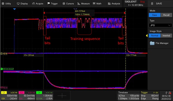
Figure 8: Histogram of Tx signal with 1-sec persistence
Peak current of almost 2 A at 4 V DCin covers the demand of the Tx power amplifier. During the reception of a call, the peak current is 100 mA. There is no measurable power consumption between the Rx paging reception, the implemented Eco-Mode only powers the 32 kHz clock inside the phone to wake-up the phone for the next paging. That’s why the battery charge can last for many days if no calls performed.
Large memory depth of the scope was very helpful to zoom-in into the captured data. Various trigger options helped to get a stable trigger for fast-changing signals.
We were extremely surprised by the good performance and rich features of the new Siglent SDS2000x Plus oscilloscope. The performance of this mid-class entry model is on the level of high-end units back in the time when one of the authors designed the A36 phone. We recommend this scope to all interested readers and look forward to checking LTE and 5G phones with this scope in our next projects.
Products Mentioned In This Article:
- SDS2000X Plus series please see HERE
Programming Example: Retrieve data from an XE series Oscilloscope using Kotlin
The SDS series of oscilloscopes all feature remote programming and data collection capabilities. They can be integrated easily into many automated test environments to ease the setup and data acquisition during testing.
One of our helpful customers developed a nice programming example designed to set up and retrieve data from a SIGLENT SDS1202X-E Oscilloscope using Kotlin, a free open source coding environment (more on Kotlin here).
The code utilizes a LAN connection and open sockets.
Thanks to Chris Welty for the code!
Here is a text file of the example:
/**
* License: 3-Clause BSD
*
* Copyright 2018 Chris Welty
*
* Redistribution and use in source and binary forms, with or without modification, are permitted provided that the following conditions are met:
*
* 1. Redistributions of source code must retain the above copyright notice, this list of conditions and the following disclaimer.
*
* 2. Redistributions in binary form must reproduce the above copyright notice, this list of conditions and the following disclaimer in the documentation and/or other materials provided with the distribution.
*
* 3. Neither the name of the copyright holder nor the names of its contributors may be used to endorse or promote products derived from this software without specific prior written permission.
*
* THIS SOFTWARE IS PROVIDED BY THE COPYRIGHT HOLDERS AND CONTRIBUTORS “AS IS” AND ANY EXPRESS OR IMPLIED WARRANTIES, INCLUDING,
* BUT NOT LIMITED TO, THE IMPLIED WARRANTIES OF MERCHANTABILITY AND FITNESS FOR A PARTICULAR PURPOSE ARE DISCLAIMED. IN NO
* EVENT SHALL THE COPYRIGHT HOLDER OR CONTRIBUTORS BE LIABLE FOR ANY DIRECT, INDIRECT, INCIDENTAL, SPECIAL, EXEMPLARY, OR
* CONSEQUENTIAL DAMAGES (INCLUDING, BUT NOT LIMITED TO, PROCUREMENT OF SUBSTITUTE GOODS OR SERVICES; LOSS OF USE, DATA, OR
* PROFITS; OR BUSINESS INTERRUPTION) HOWEVER CAUSED AND ON ANY THEORY OF LIABILITY, WHETHER IN CONTRACT, STRICT LIABILITY,
* OR TORT (INCLUDING NEGLIGENCE OR OTHERWISE) ARISING IN ANY WAY OUT OF THE USE OF THIS SOFTWARE, EVEN IF ADVISED OF THE
* POSSIBILITY OF SUCH DAMAGE.
*/package scope
import java.io.BufferedWriter
import java.io.OutputStreamWriter
import java.io.Serializable
import java.net.Socket/**
* Contains a single waveform downloaded from a Siglent 1202X-E
*/
class Waveform(val vDiv: Double, val vOffset: Double, val tDiv: Double, val tOffset: Double, val data: ByteArray) : Serializable {val xs: DoubleArray
get() = DoubleArray(data.size, { i -> i * tDiv * 14 / data.size + tOffset – tDiv * 7 })val ys: DoubleArray
get() = DoubleArray(data.size, { i -> data[i] * vDiv / 25 – vOffset })companion object {
/**
* Download the waveform displayed on the scope’s screen
*/
fun download(): Waveform {
Socket(“192.168.1.222”, 5025).use { socket ->println(“connected to ” + socket.inetAddress)
val output = BufferedWriter(OutputStreamWriter(socket.getOutputStream(), Charsets.US_ASCII))// since the socket can return binary data, we can’t use an InputStreamReader to
// translate the bytes to characters. We’ll have to do it ourselves.
// SCPI generally uses US ASCII, shouldn’t be too hard.
val input = socket.getInputStream()/**
* Read from the scope until \n is encountered.
* The bytes are translated to characters numerically (so US_ASCII).
*/
fun readLine(): String {
val sb = StringBuilder()
while (true) {
val c = input.read()
when (c) {
-1, ‘\n’.toInt() -> return sb.toString()
else -> sb.append(c.toChar())
}
}
}/**
* Read a number of bytes from the scope.
*
* The bytes are not translated into characters.
*/
fun readBytes(n: Int): ByteArray {
val result = ByteArray(n)
var i = 0
while (i < n) {
i += input.read(result, i, n – i)
}
return result
}fun writeLine(string: String) {
output.write(string)
output.write(“\n”)
output.flush()
}/**
* Read a numerical response from the scope.
*
* The scope returns responses like “C1:VDIV 1.00E+00V”.
* This function extracts the “1.00E+00″, converts it to a double, and returns it.
*/
fun readNumber() = readLine().split(” “)[1].dropLast(1).toDouble()writeLine(“*IDN?”)
println(readLine())// reset the scope response format to its default so readNumber() works
writeLine(“CHDR SHORT”)writeLine(“C1:VDIV?”)
val vDiv = readNumber()writeLine(“C1:OFST?”)
val vOffset = readNumber()writeLine(“TDIV?”)
val tDiv = readNumber()writeLine(“TRDL?”)
val tOffset = readNumber()// request all points for the waveform
writeLine(“WFSU SP,0,NP,0,F,0”)
writeLine(“C1:WF? DAT2”)// parse waveform response
val header = String(readBytes(21))
println(“header is $header”)
val length = header.substring(13, 21).toInt()
println(“length is $length”)
val data = readBytes(length)
readBytes(2) // 2 garbage bytes at endprintln(“V/div = $vDiv; offset = $vOffset; t/div = $tDiv; tOffset = $tOffset”)
return Waveform(vDiv, vOffset, tDiv, tOffset, data)
}
}
}
}Products Mentioned In This Article:
Siglent Oscilloscopes please see HERE
Comparison / Differences between the SDS1000X and SDS1000X-E oscilloscope families
The short list of differences between the X and the 2 channel XE (SDSs1202XE) is as follows:– X has 50 ohm/ 1 MOhm selectable input impedance. XE only has 1 MOhm fixed. You will need a 50 ohm matching through adapter if you wish to connect to 50 Ohm circuits/minimize reflections.– The X has a slightly larger display (8″) vs. the XE (7″)– The XE has a faster digital platform with 1 Mpt FFT capability. The X has 16,384 pt depth for the FFT.In addition, the SDS1xx4X-E scopes have additional differences:– Onboard webpage control (standard)– Bode Plot (standard.. requires SIGLENT SDG or SAG1021)– External waveform/function generator (SAG1021 and SDS1000X-E-FG license Optional)– WiFi control (TL-WN725N and SDS1000X-E-WiFi license Optional)Products Mentioned In This Article:Programming Example: List connected VISA compatible resources using PyVISA
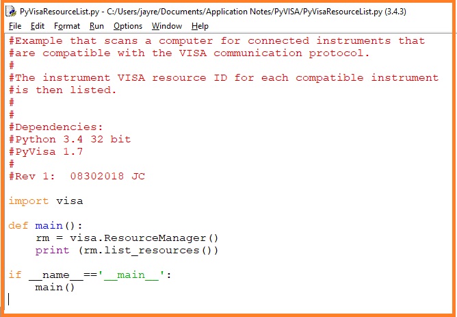
PyVISA is a software library that enables Python applications to communicate with resources (typically instruments) connected to a controlling computer using different buses, including: GPIB, RS-232, LAN, and USB.
This example scans and lists the available resources.
It requires PyVISA to be installed (see the PyVISA documentation for more information)
***
#Example that scans a computer for connected instruments that
#are compatible with the VISA communication protocol.
#
#The instrument VISA resource ID for each compatible instrument
#is then listed.
#
#
#Dependencies:
#Python 3.4 32 bit
#PyVisa 1.7
#
#Rev 1: 08302018 JCimport visa
def main():
rm = visa.ResourceManager()
print (rm.list_resources())if __name__==’__main__’:
main()
*****
Here is the code:
And here is the result of a scan:
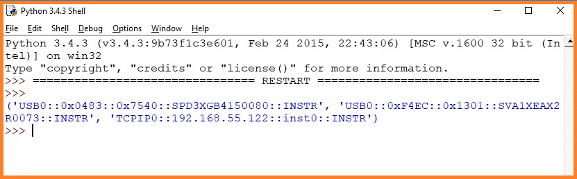
Each connected instrument returns a specific formatted string of characters called the VISA Resource ID.
The resource ID format is as follows:
‘Communication/Board Type (USB, GPIB, etc.)::Resource Information (Vendor ID, Product ID, Serial Number, IP address, etc..)::Resource Type’
In the response, each resource is separated by a comma. So, we have three resources listed in this example:
‘USB0::0x0483::0x7540::SPD3XGB4150080::INSTR’ – This is a power supply (SPD3X) connected via USB (USB0)
‘USB0::0xF4EC::0x1301::SVA1XEAX2R0073::INSTR’ – This is a vector network analyser (SVA1X) connected via USB (USB0)
‘TCPIP0::192.168.55.122::inst0::INSTR’ – This is an instrument connected via LAN using a TCPIP connection at IP address 192.168.55.122
Products Mentioned In This Article:
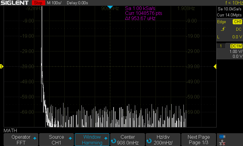
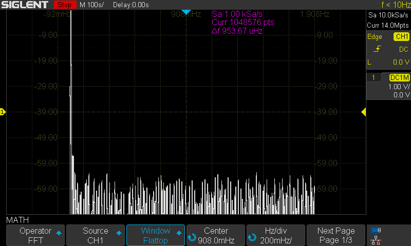
SDS FFT performance on low frequency signals
Like many modern oscilloscopes, the SIGLENT SDS series feature FFT math functions that calculate frequency information from the acquired voltage vs. time data. FFT stands for Fast Fourier Transform, and is a common method for determining the frequency content of a time-varying signal. Converting time domain data to the frequency domain makes measuring characteristics like phase noise and harmonics much easier. Oscilloscopes don’t have the dynamic range or sensitivity of a true spectrum analyser, but these new designs can provide a fine level of detail that may be just enough for your application.
FFTs are commonly used on high frequencies, but they can also be used on signals with fairly low frequencies.
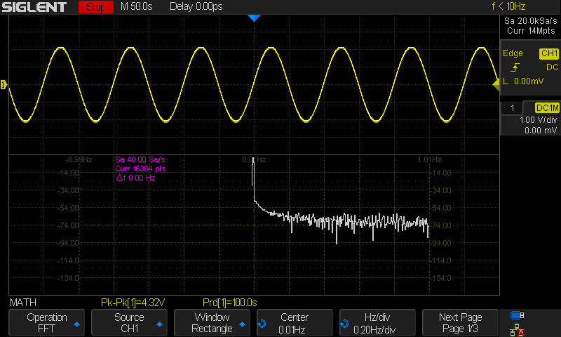
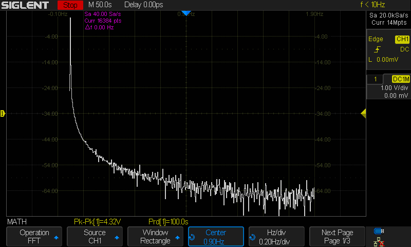
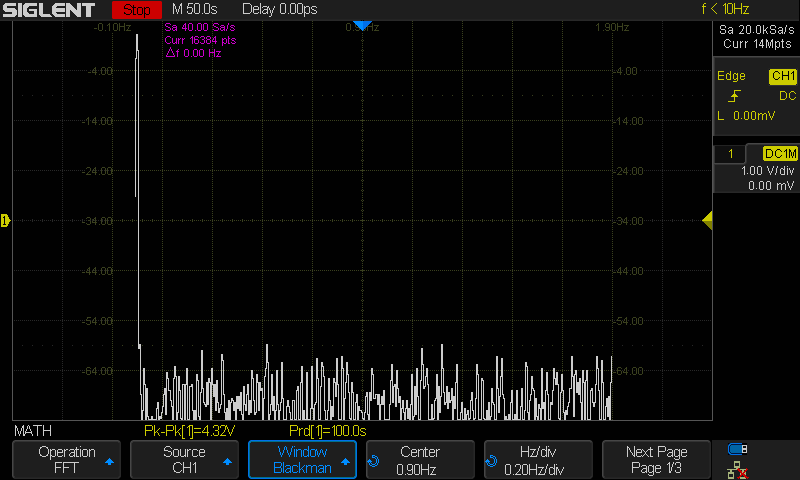
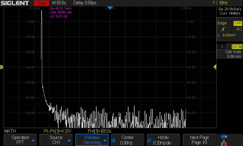
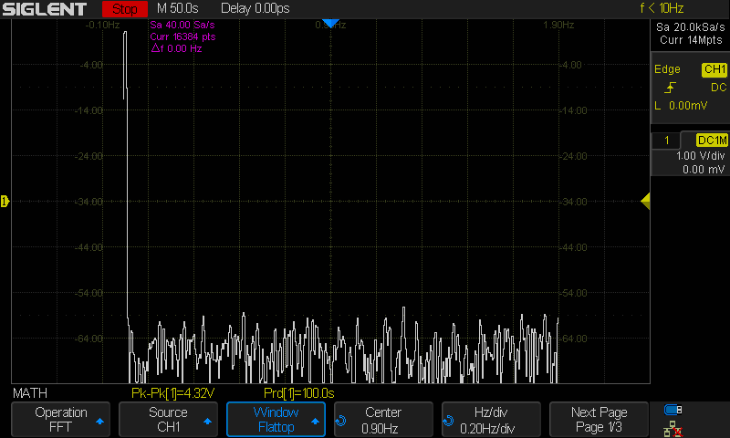
In this note, I am going to show the FFT performance of two series of our scopes by sourcing a 10 MHz (100 s period), 10 Vpp sine wave using a SIGLENT SDG805 Function Generator into Channel 1.
SDG805 has been discontinued, to see other models in the SDG800 series please click HERE
SDS1000X/SDS2000X Series:
The SDS1000X and 2000X series feature an FFT function that uses up to 16 kpts of timebase data to calculate the frequency data and a timebase maximum of 50 s/div.
Here are the FFT results with the available window settings for a 10 MHz sinewave –
The scope can show a split timebase and FFT view:
For the rest, I will use the exclusive FFT view.
Rectangle
Blackman
Hanning

Hamming
Flat Top
SDS1000X-E Series:
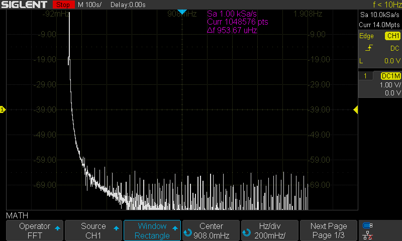
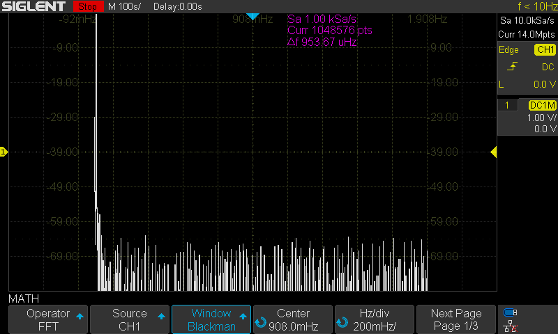
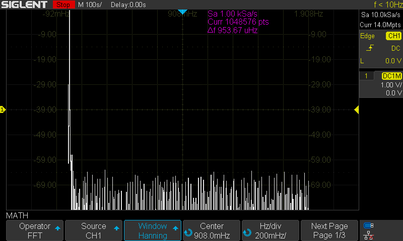
The SDS1000X-E series feature a new math co-processor that increases the maximum data depth of the FFT function to 1 Mpts. They also feature a timebase maximum of 100 s/div. These increases allow the X-E to have much finer timebase detail and to acquire useful data for even lower frequencies than many scopes on the market.
Here are the FFT results with the available window settings for a 10 MHz sinewave –
The scope can show a split timebase and FFT view:
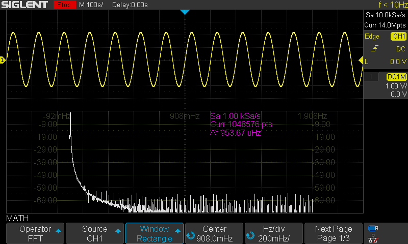
For the rest, I will use the exclusive FFT view.
Rectangle
Blackman
Hanning
Hamming
Flat Top
Products Mentioned In This Article: