Your cart is currently empty!
Author: James

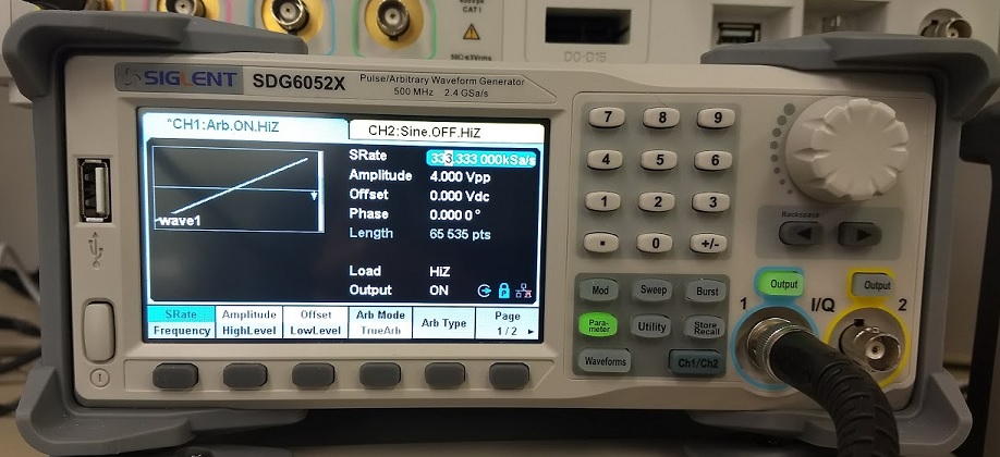
Python Example: Building an Arb with 16-bit steps (SDG2000X/SDG6000X)
The SIGLENT SDG2000X and SDG6000X feature 16-bit voltage step resolution. This provides 65,535 discrete voltage steps that can cover the entire output range (20 Vpp into a High Z load) which can effectively be used to test A/D converters and other measurement systems by sourcing waveforms with very small changes.
In this example, we use Python 2.7 and PyVISA 1.8 to create a ramp waveform that is comprised of steps of the Least Significant Bit (LSB) from point 0 to 65535 on Channel 1.
We also implement the TrueArb function that allows you to specify the sample rate and also ensures that each sample is sourced.
NOTE: You will need to change the instrument ID to match your specific instrument. We also recommend setting the amplitude and other instrument parameters prior to enaling the output of the instrument.
Here is pic of the instrument after loading the waveform:
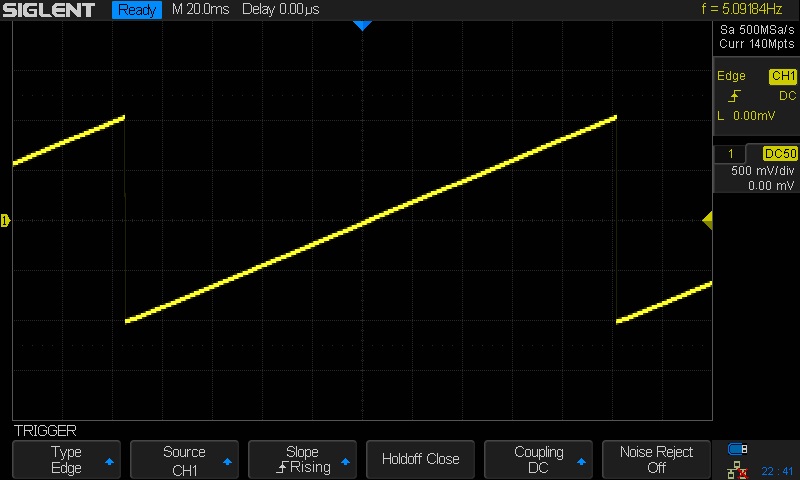
Here is a scope shot of the output:
Here is a link to a Zipped version of the .PY file: SiglentSDG16BBitSteps
Here is the text of the program:
##
#!/usr/bin/env python2.7
# -*- coding: utf-8 -*-
import visa #Uses PyVISA 1.8 and NI-VISA runtime Engine 15.5
import time
import binascii#USB resource of Device
rm = visa.ResourceManager()
device = rm.open_resource(‘USB0::0xF4EC::0x1101::SDG6XBAQ1R0071::INSTR’) #CHANGE TO MATCH YOUR INSTRUMENT ID#Little endian, 16-bit 2’s complement
# create a waveformwave_points = []
for pt in range(0x8000, 0xffff, 1):
wave_points.append(pt)
wave_points.append(0xffff)
for pt in range(0x0000, 0x7fff, 1):
wave_points.append(pt)def create_wave_file():
#create a file
f = open(“wave1.bin”, “wb”)
for a in wave_points:
b = hex(a)
#print ‘wave_points: ‘,a,b
b = b[2:]
len_b = len(b)
if (0 == len_b):
b = ‘0000’
elif (1 == len_b):
b = ‘000’ + b
elif (2 == len_b):
b = ’00’ + b
elif (3 == len_b):
b = ‘0’ + b
b = b[2:4] + b[:2] #change big-endian to little-endian
c = binascii.a2b_hex(b) #Hexadecimal integer to ASCii encoded string
f.write(c)
f.close()def send_wave_data(dev):
#send wave1.bin to the device
f = open(“wave1.bin”, “rb”) #wave1.bin is the waveform to be sent
data = f.read()
print (“write bytes:”,len(data))
dev.write_raw(“C1:WVDT WVNM,wave1,FREQ,2000.0,TYPE,8,AMPL,4.0,OFST,0.0,PHASE,0.0,WAVEDATA,%s” % (data))
#”X” series (SDG1000X/SDG2000X/SDG6000X/X-E)
dev.write(“C1:ARWV NAME,wave1”)
f.close()if __name__ == ‘__main__’:
create_wave_file()
send_wave_data(device)
device.write(“C1:SRATE MODE,TARB,VALUE,333333,INTER,LINE”) #Use TrueArb and fixed sample rate to play every point###
DIY Spectrum Analyser Input Protection
Spectrum analysers like the SIGLENT SSA3000X and SVA1000X series are extremely useful instruments that can provide invaluable insight into broadcast signal performance, transmitter troubleshooting, and interference as well as RF device characterization and EMC testing.
But, like other spectrum analysers, they are very sensitive and can be damaged easily, if the proper precautions are not followed.
The instruments have standard protection elements that includes a DC blocking capacitor and an automatic attenuator that help to prevent damage from low frequency and higher powered signals. There is even an audible and visible warning if the ADC (Analog-to-Digital Converter) overload.
In addition to this, adding external attenuation and protection can be useful in further preventing damage, especially when connecting to unknown sources such as antennas, transmitters, and LISNs.
One of our customers, Mr. Jeff Covelli (WA8SAJ), is a HAM (Amateur Radio Operator) who recently shared a very simple protection box that can be useful for keeping that sensitive front end functioning when connecting to unknown signal sources.
He uses it to help protect the input on his SIGLENT SDG1032X signal generator as well as his SSA3021X spectrum analyser:
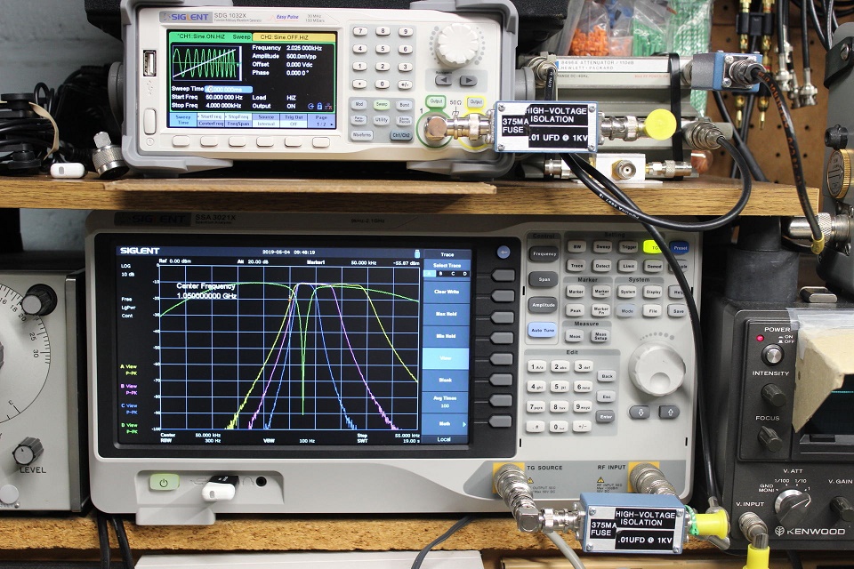
And he has a pretty impressive setup:
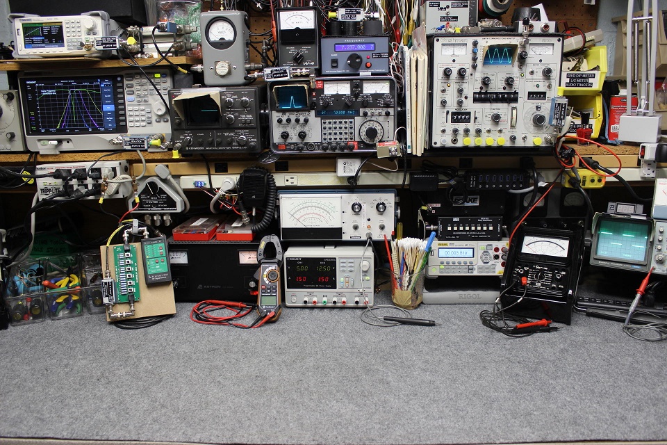
And here are the details:
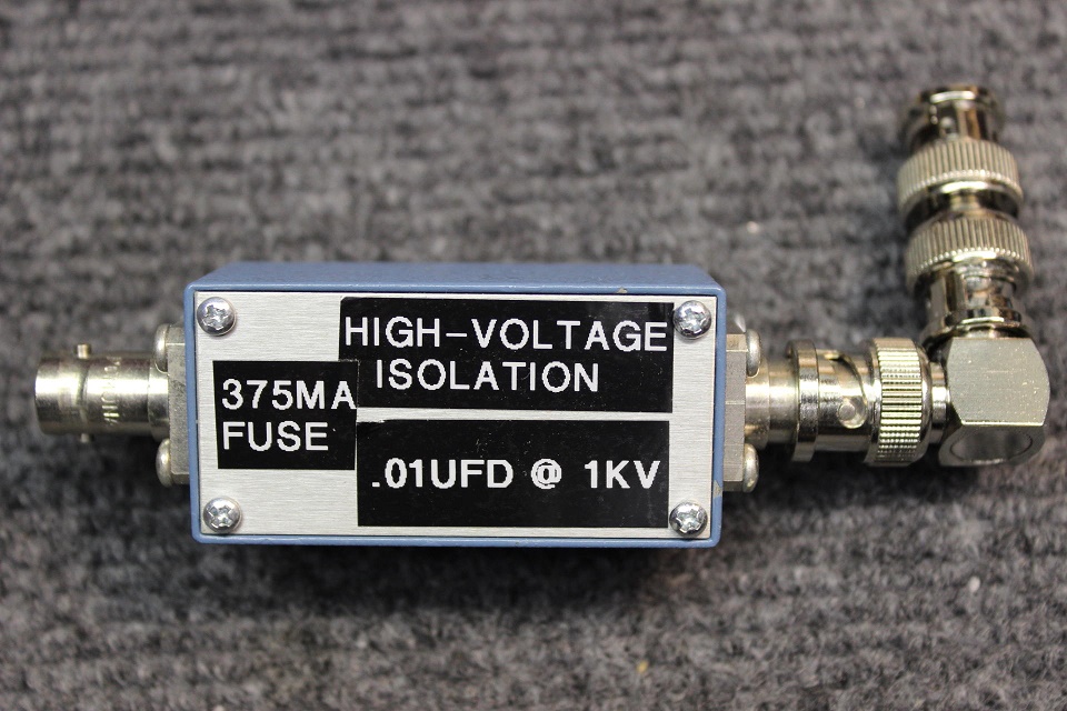
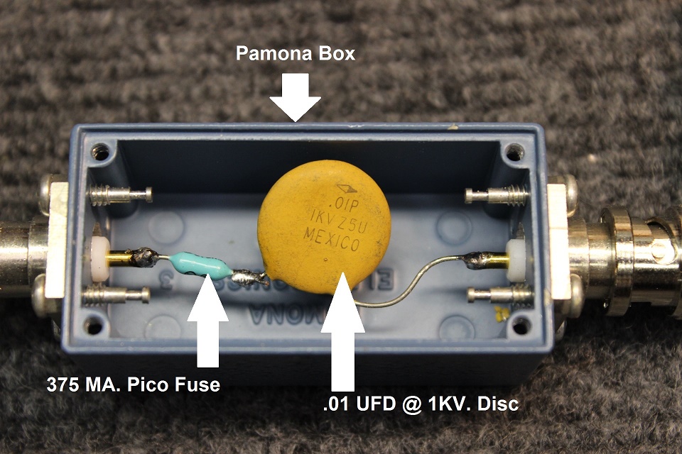

At some point, I hope to characterize this setup and provide S11, S21 information.. but, if your signal is unknown, this will add an additional layer of protection when measuring an unknown signal for the “first time”.
Two-tone testing: Building an arbitrary waveform using the Equation Draw function
In this note, we are going to use Equation Draw within EasyWave to create a waveform that is built using the addition of sine waves with two different frequencies (700 and 1900 Hz). We will then show how to use this signal to modulate a carrier up-to 500 MHz using the other SDG output channel.
EasyWave is free software designed to help create and edit arbitrary waveforms and download them to applicable SIGLENT SDG series of arbitrary waveform generators, including the SDG800, 1000, and X series. You can download it here: EasyWave
EasyWave has an interesting feature called Equation Draw that enables you to create complex waveforms using some common basic math and trigonometric functions, like +, -, *, /, sine, cosine, and more.
NOTE: Two-tone testing is commonly used to test the performance of audio data that is embedded in modulated signals like AM or FM radio broadcasts. You can use two-tone signals to check the performance of RF receivers. The ARRL and other radio-centric organizations have lots of data on testing receivers, for those so inclined.
Many of the SDG products have a wave combine feature that mathematically adds the waveforms for both channel 1 and channel 2. This is technically easier than the process we highlight in this note, but it requires the use of both channels of the SDG. The using a single output arbitrary waveform allows us to use the other free channel for other tasks, including sourcing a carrier modulated by our two-tone signal (see the end of this note for more info).
To learn about Wave Combine, click here: Wave Combine
Setup
- SIGLENT SDG arbitrary waveform generator (We are using an SDG6052X capable of 500 MHz for this note)
- EasyWave software
- USB or LAN connection
Before beginning, please install EasyWave (The instructions are available with the download available here: SDG Software Downloads) and connect the instrument to the computer.
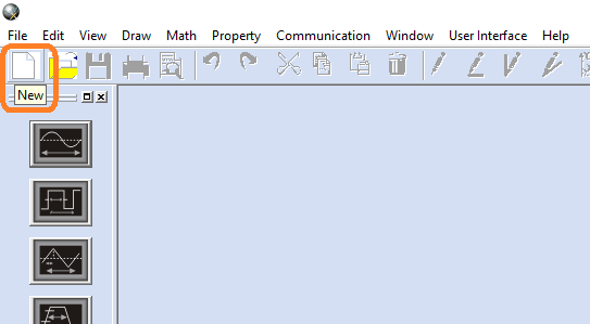
- Open EasyWave by double-clicking on the EasyWave Icon:

2. Open a new waveform:
3. Name the waveform (optional) and set the frequency of the main repeated waveform. In this case, we will set the Frequency to 100 Hz. Press OK:
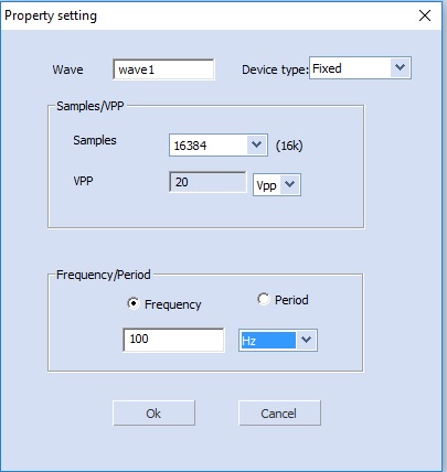
NOTE: The arbitrary waveform “frequency” is the repetition frequency of the entire waveform loaded into memory. If that waveform has a single period, then the set frequency here will be the frequency of the output waveform. If the waveform has 2 periods, then this frequency will be half of the actual waveform frequency (because there are 2 periods per memory “frame”). In this process, the frequency set in this step is equal to the “X” variable used in future steps.
4. This opens the wave1 waveform window. Now, click on the Equation Draw icon to open the equation editor. This includes a listing of available math elements as well as a saved equations area.
For this example, we want two tones… one at 700 Hz and the other at 1900 Hz. Since we set the output frequency to 100 Hz (remember we named that “X” above), we can simply enter our equation in the New Equation field using standard trigonometric functions as shown:
y(x) = sin(7*x) += sin(19*x)
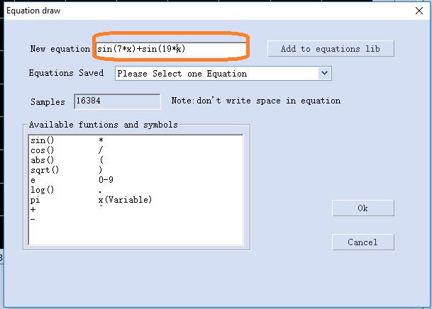
Press OK to enter.
NOTE: This will create a waveform that is the addition of two sine waves. One with a frequency 7 times X (7*100 Hz = 700 Hz) and the other with a frequency 19 times X (19*100 Hz = 1900 Hz).
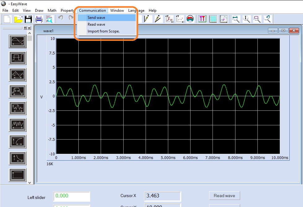
Now, the wave window shows a green waveform that represents the waveform we entered via the Equation Draw method. Confirm that it matches your expectations for your application.
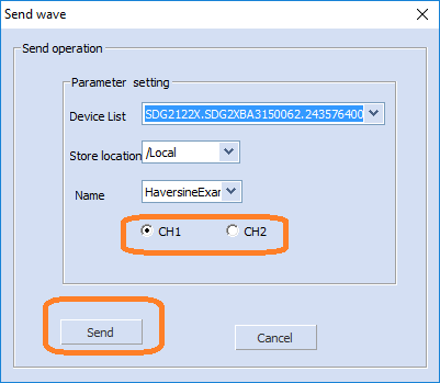
5. Press Communication to open the dialog to begin downloading the waveform to the instrument:

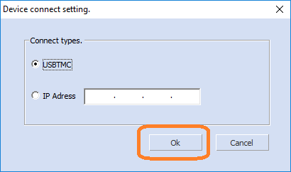
6. Select the connection type (USB = USBTMC) and press OK
7. Select the correct USB device, Waveform Name, and Channel.. press OK:
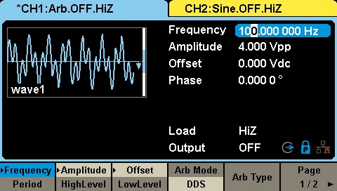
8. Now, you can observe the waveform and parameters on the display of the generator. Here, you can change the base frequency, amplitude, and other waveform characteristics.
Here is a screen capture of an oscilloscope using the FFT function to capture the spectral content of the output using the waveform created:
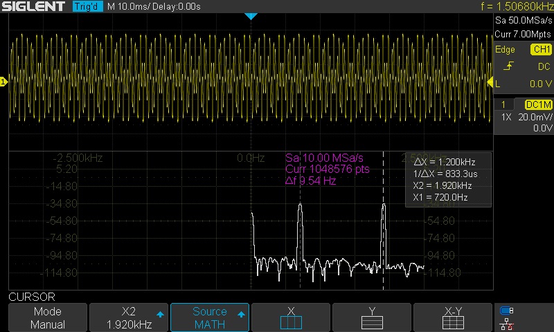
Note that the frequency markers show peaks at 700 and 1900 Hz, as expected.
Next Step: Source a two-tone modulated carrier
Now that we have verified the two-tone output, we can use this waveform as a modulation source for a higher frequency carrier. This modulated signal can be used to test the performance of a receiver.
Here are two options for creating a modulated carrier:
SDG External Modulation for carriers < 500 MHz
Many SDG generators include an external modulation input which can be used to modulate the output of a specified channel. In this example, we can simply route the two-tone channel to the external modulation input. Then, configure the other channel to output a modulated carrier.
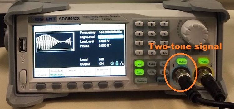
Here, we will use the SDG6052X, which can output sine waves up to 500MHz. As mentioned previously, this technique works with any dual channel SDG. When selecting a generator, remember that the maximum carrier output frequency includes the modulation bandwidth. If your generator has a maximum frequency of 100 MHz and the modulation bandwidth is 10 kHz, then the maximum carrier frequency when modulation is active will be 100 MHz – 10 kHz/2.
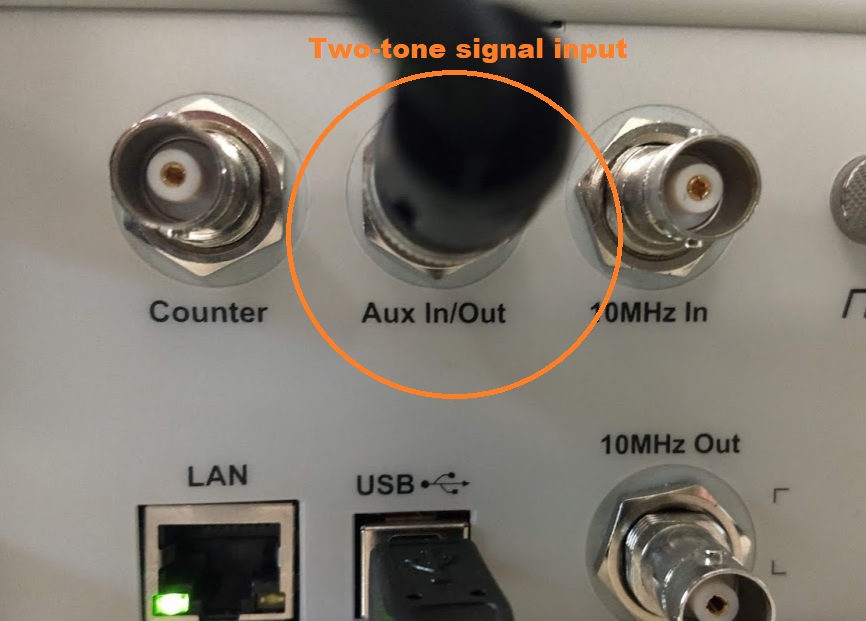
- Route a cable from the two-tone channel to the Aux In located on the rear panel. In this case, channel 1 is the two-tone source:
Front Panel:
Rear Panel:
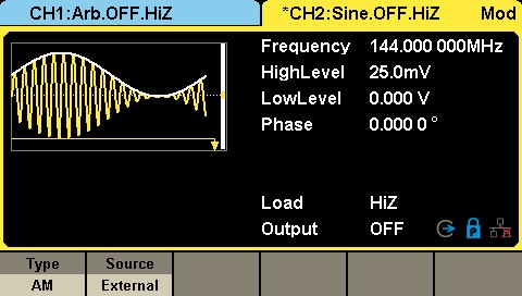
- Configure the other channel as the modulated carrier (channel 2, in this example) for external modulation by pressing Mod and configuring the channel as shown.
Here, we set the channel to use the external input to modulate an AM carrier with a frequency of 144 MHz, in the amateur radio broadcast 2m band :
Now, we can confirm the output using a spectrum analyser.
Here, we connect the modulated carrier output (channel 2) into a SIGLENT SVA spectrum analyser:
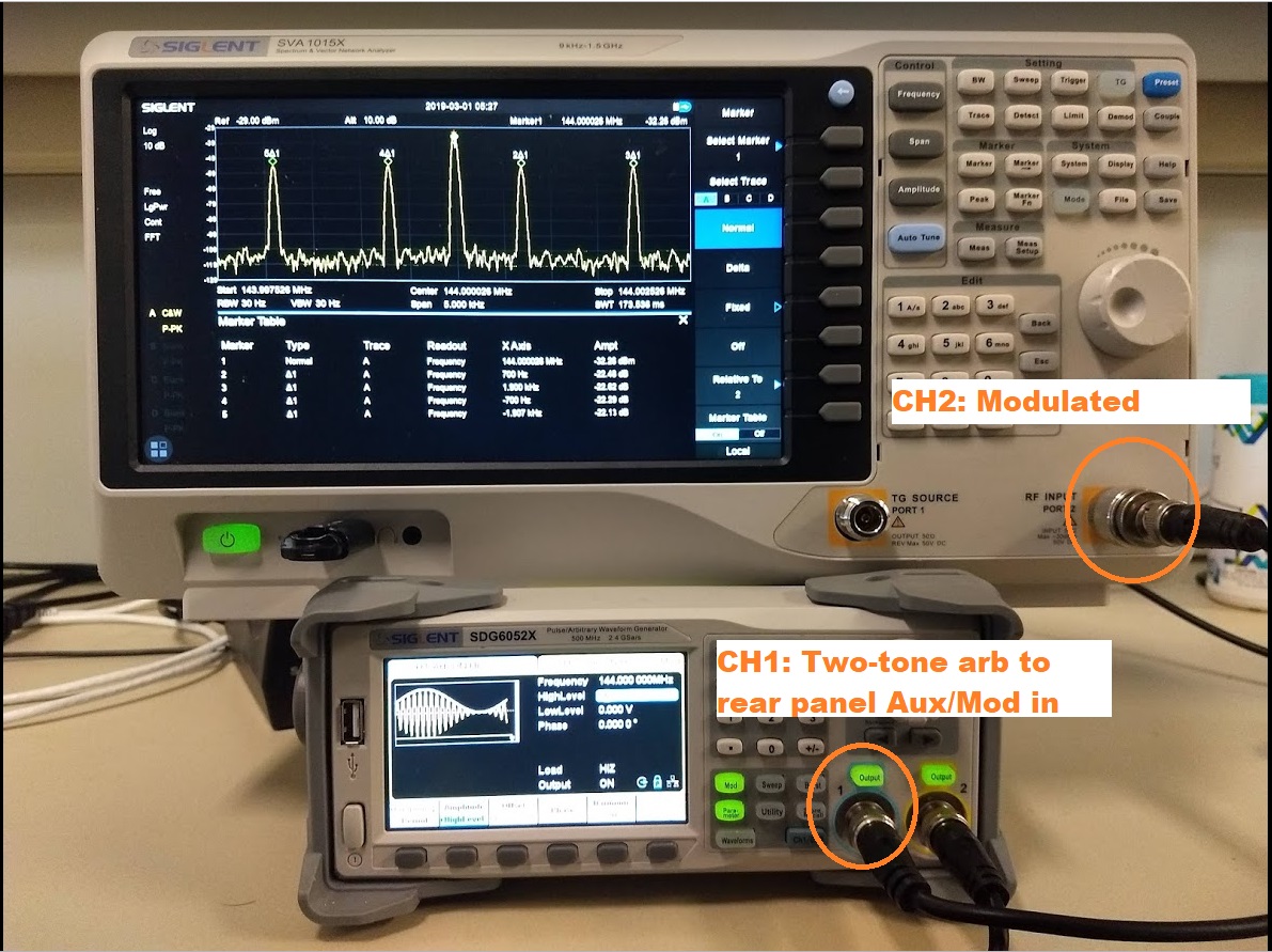
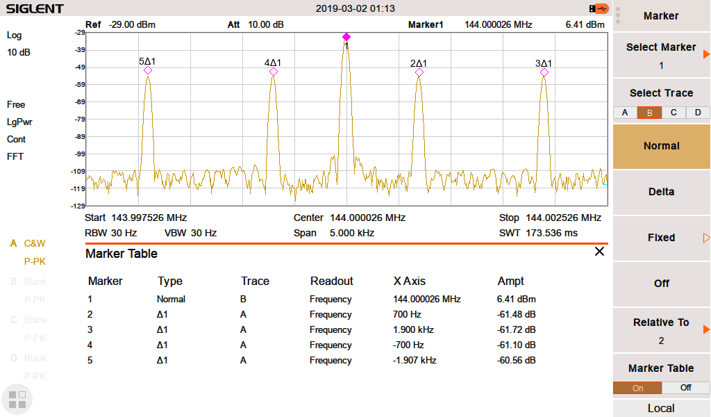
Here, you can see the carrier at 144 MHz, and the two tones at +700, +1900, -700, and +1900 Hz from the carrier.. as expected.
NOTE: Make sure that the output power of your SDG is low enough to prevent damage to the spectrum analyser or add enough external attenuation to make sure you don’t damage the input.

Testing Open Socket Communications Using PuTTY
Many instruments include the ability to be controlled via a remote connection to a computer using an Ethernet connection. In many cases, these instruments require a special software library that can help establish and maintain the communications link between the instrument and controlling computer. This can be annoying for a few reasons… the software library is likely to occupy a large amount of space on the controlling computer and is also required on any computer that is being used to control the instrument. In a remote networking application where multiple user’s may want access to a test instrument, this can cause support and installation headaches.
Luckily, there are a few solutions that can help. In this application note, we are going to discuss using open socket communication techniques using an open source communication tool called PuTTY with a SIGLENT SSA3032X spectrum analyser.
What are open sockets and why use them?
Within the context of Ethernet/LAN connections, sockets are like mailboxes. If you want to deliver information to a specific place, you need to be sure that your information is delivered to the correct address.
In the context of test instrumentation, an open socket is a fixed address (or port number) on the Ethernet/LAN bus that is dedicated to process remote commands.
Open sockets allow remote computers to simply use existing raw Ethernet connections for communications without having to add additional libraries (VISA or similar) that require additional storage space and processing overhead.
Programs that utilize sockets for LAN communication tend to take up less memory and operate more quickly.
PuTTY
PuTTY is an open source software tool that provides a number of simple communication links (RAW, Telnet, SSSH, Serial, and others). It is available for free and there are a number of versions available for popular operating systems.
You can download as well as learn more here: https://www.putty.org/
In this example, we are using PuTTY to verify the raw LAN connection is working properly. It is quite a simple program that does not allow for very complex operation (sequences, converting data sets/strings, etc..). If you require more complex functionality, software platforms like Python, .NET, C#, LabVIEW, etc.. can be used to control the instrument using a similar open socket connection.
Configuration
In this test, we are using the most current revision of the SIGLENT SSA3032X Spectrum Analyzer firmware (Revision 01.02.08.02) which enables open socket communication.
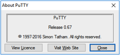
This example also uses PuTTY version 0.67:
Steps
1. Install PuTTY for the OS you intend to use
2. Make sure your instrument and firmware revision can use open sockets
The SSA3032X revision 01.02.08.02 enables open socket communication.
To find the revision, press the System button > Sys Info.
Figure 1 below shows a sample system information screen from a SIGLENT SSA3000X analyzer:
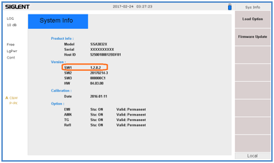
Figure 1: Sample system information page from an SSA3000X.Check the product page and firmware release notes for more information.
3. Connect the instrument to the local area using an Ethernet cable
4. Find the IP address for the instrument. This is typically located in the System Information menu. On the SIGLENT SSA3032X, press the System button on the front panel > Interface > LAN.
Figure 2 below shows a sample LAN setup page from a SIGLENT SSA3000X:
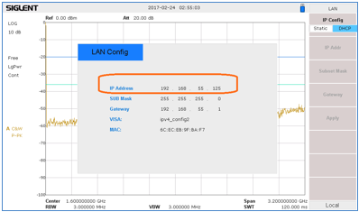
Figure 2: Sample LAN information page from an SSA3000X.5. Open PuTTY
6. Select Raw as connection type
7. Enter the IP address in the Host Name field
8. Enter the port number. This should be provided in the users or programming guide for the instrument.
The SIGLENT SSA3000X uses port 5025.
Figure 3 below shows the PuTTY configuration for this example:
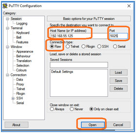
Figure 3: Example PuTTY configuration.9. Press Open. This will open a terminal window as shown in below:
10. Using the computer keypad, enter *IDN? and press the Enter key on the keyboard to send the command.
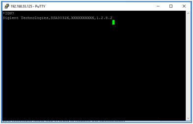
This is the standard command string that is used to request the identification string from the instrument. As shown below, the instrument responds with the manufacture, product ID, Serial Number, and firmware revision.
Conclusion
PuTTY is an easy way to verify an operational LAN connection to instrumentation that can use open sockets.
Quick remote computer control using LXI Tools
Introduction:
There are many options for people considering remote communication and control of test and measurement instrumentation. In most cases, a computer is used to communicate to test instrumentation using USB or LAN connections. The computer can configure the instruments, collect and organize data, and present it in a useful and flexible way.
Remote control provides:
- Increased repeatability: The instrumentation is set up the same way, every time.
- Efficient data collection: Data can be automatically filtered and stored.
- Easily configure the test system parameters: Each command is executed in the same order and in the same timeframe.
- Quickly visualize system performance: Graphical or tabular data formatting is easy.
There are numerous platforms (Windows, Linux, etc..) and software programs (LabVIEW, .NET, Python) available to build automated test systems. The right choice for your application is highly dependent on your needs and the available skills you have.
In this note, we are going to discuss how to use LXI Tools to communicate with SIGLENT instrumentation. LXI Tools is an open source software application that uses the local area network (LAN) connection to quickly control remote instrumentation. It is easy to install, has a small operating footprint, and is really powerful while being quite easy to use. Let’s start by looking at the basics.
You can also see the video version of this note here: https://siglentna.com/video/lxi-tools/
Why Open Source?
Open source coding is a community-based development style in which a group of contributors work together to build and maintain programs using shared code and components. In this way, a platform can be built and tested quickly and may cost significantly less than commercial programming environments. LXI Tools is free open source software and the project welcomes new contributors that would like to help improve the tools.
Here is a link to the LXI Tools website: https://lxi-tools.github.io
Why LXI Tools?
LXI-Tools is a collection of open source software tools that provide direct control of LXI compatible instruments such as modern oscilloscopes, power supplies, spectrum analyzers, and more.Simply install LXI Tools, connect your instrument, and start communicating.
It really is that easy.
LXI-Tools Provides:
- Quickly discover the available instruments on the LAN
- Retrieve copies of the displayed images (quickly see signals, data, and instrumentation setups) and convert image file types
- Benchmark LAN performance
- Send individual commands to an instrument to perform simple test actions. For example, you could return the measured data from a DMM.
To learn more about LXI-Tools, please see https://github.com/lxi-tools/lxi-tools
Instructions:
- Install the appropriate version of LXI-Tools for your operating system
2. Open a terminal. In this example, I am using Ubuntu (17.10) running on a virtual machine hosted by a Win 10/64 bit OS.
To learn more about the virtual machine used in this example:https://www.virtualbox.org/
The OS is Ubuntu: https://www.ubuntu.com/
3. Once loaded, startup Linux:
With Ubuntu, you can use Snap to install:
$ snap install lxi-tools
LXI Discover:
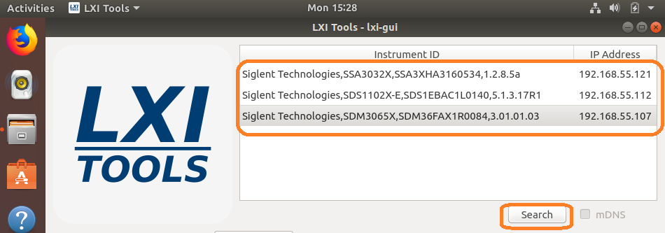
Quickly searches the LAN for instruments and lists their identification string and IP address.
Plug in and power on your instrumentation and make sure that they are connected to a working LAN connection. You can manually check the instrument IP address and save this info to compare to later steps.
Open up a terminal window. At the “$” prompt, simply type lxi discover… LXI tools will search the LAN for connected instruments.
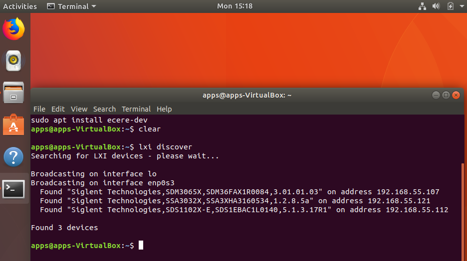
Here, we have three devices connected: an SDM3065X, SSA3032X, and an SDS1102X-E (which has been superseded by the SDS1202X-E series here in North America). It also includes the instrument serial number, firmware revision, and IP address.
NOTE: This has been tested with a large number of instruments, but may not be supported by some. There is a list of compatible instruments at the end of this note or you can check LXI-Tools support for the latest list of supported products.
Screenshot:
This function retrieves a copy of the instrument display and saves it to the local drive. This is ideal for adding information to reports and sharing events with colleagues.
Type “lxi screenshot – – address <device address>”
NOTE: There should be two “-” with no spaces before “address” for every command.

Image Edits using ImageMagicks
Use ImageMagick® to create, edit, compose, or convert bitmap images. It can read and write images in a variety of formats (over 200) including PNG, JPEG, JPEG-2000, GIF, TIFF, DPX, EXR, WebP, Postscript, PDF, and SVG. Use ImageMagick to resize, flip, mirror, rotate, distort, shear and transform images, adjust image colors, apply various special effects, or draw text, lines, polygons, ellipses and Bézier curves.
For more information, visit… https://www.imagemagick.org/script/index.php
$ lxi screenshot –address <ip> – | convert – screenshot.jpg
$ lxi screenshot –address <ip> – | convert – screenshot.tiff
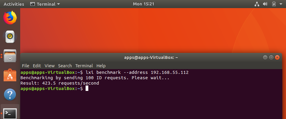
$ lxi screenshot –address <ip> – | convert – screenshot.bmpBenchmark:
The benchmark command sends 100 requests via LAN and measures the average response time of the instrument. It can be used as a gauge for the health of the connection. Higher response rates = faster links.
$ lxi benchmark –address <ip>
Manual vs. Auto-load:
The commands can also be manually or auto-loaded:
Auto-load/detect:
$ lxi screenshot –address 10.0.0.42
Vs. manually specifying which screenshot plugin to use:
$ lxi screenshot –address 10.0.0.42 –plugin siglent-ssa3000x
The only advantage of manually specifying which plugin to use it that it is a bit faster because it does not go through the instrument auto detection steps (retrieve ID, parse regex rules to match correct plugin etc.).
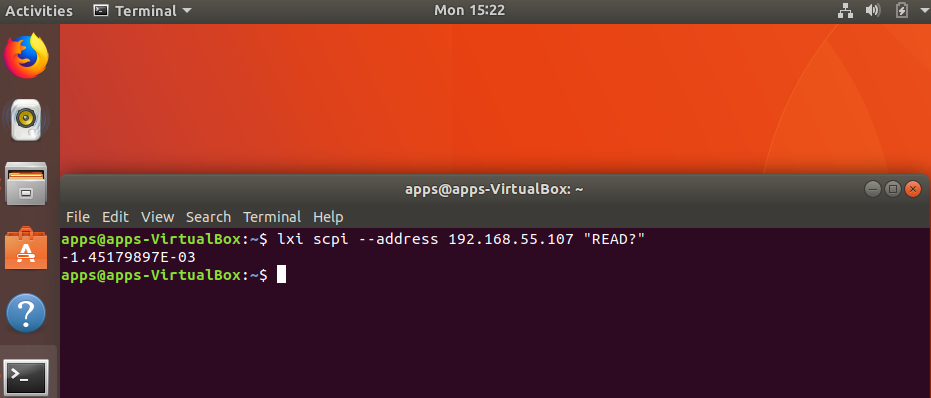
Sending instrument specific commands:
You can also use the SCPI command to send any command to the instrument.
Note that if you have an SCPI command with spaces you must remember to send the specific command in quotes like so:
$ lxi scpi –address 192.168.55.113 “MEAS:VOLT? CH1”
This way the tool knows how to parse the full SCPI string.
In this example, we send the “READ?” command to an SDM and return a reading:
GUI
Another really great feature is the GUI for LXI Tools. This allows you easy access to discovery of instruments on the network as well as some powerful tools for data capture and instrument control.
$ lxi-tools.lxi-gui
This adds a very simple yet powerful graphical interface for the LXI tools program:
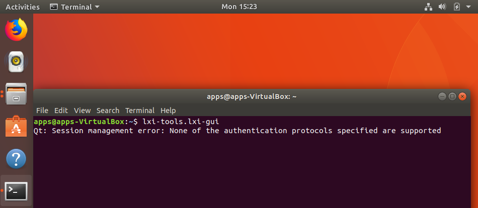
NOTE: Ignore the “Qt” error shown.
This opens a clean control window:
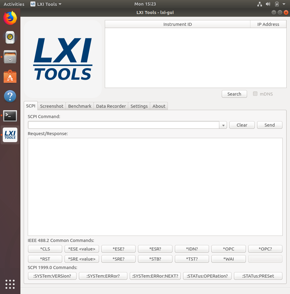
- Search: Discover the instruments connected to the LAN. Here, we have three instruments connected:
- SCPI command line: Send instrument specific commands. Click on the instrument you wish to communicate with and then enter the command. For queries (commands that require an instrument response, or read function), the returned string will be shown in the text box:
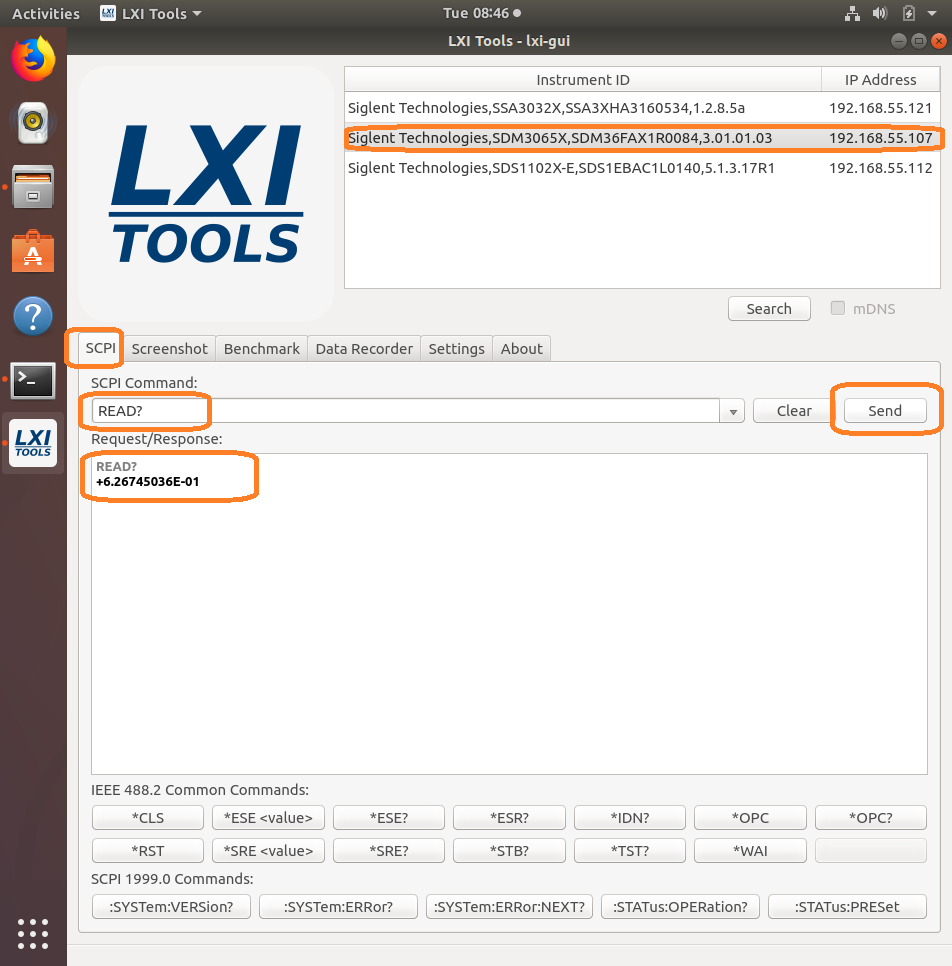
NOTE: The specific commands that can be used are available in the instrument programming guide. Check out the specific instrument documentation for more details.
This tool can be helpful when trying out specific sequences of commands. You can send them one-at-a-time and then observe the instrument functionality.
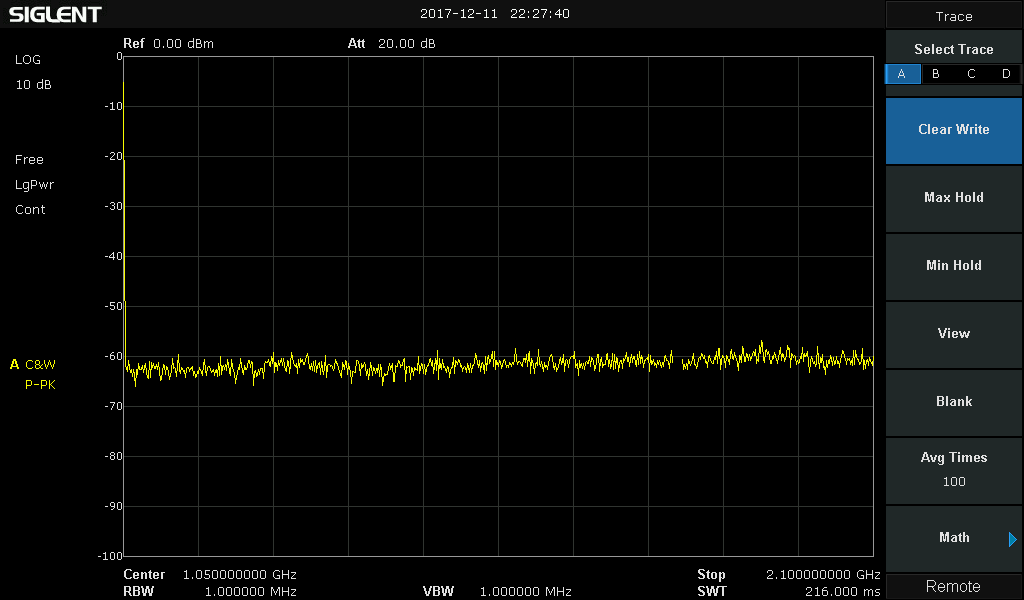
- Screenshot: Capture and save an image from the instrument. This also features a “live” button that will continuously poll the instrument.
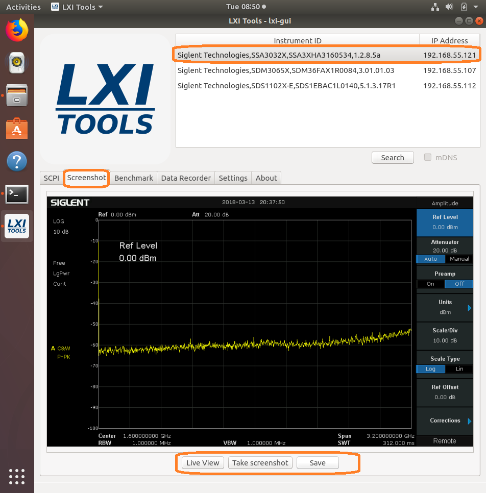
After saving, you can recall the image:
- Benchmark: Checks the performance of the LAN connection by sending a series of commands and measuring the response time. Larger “requests/second” = greater possible bus performance.
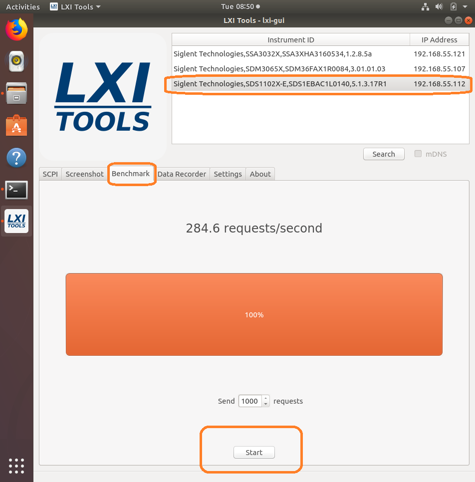
- Data Recorder: Sends the user-defined command a number of times/second and attempts to graph the data. Be aware that data can be returned in different formats and at different rates depending on device configuration. Going faster can make the system unstable and could cause a crash or hang-up.
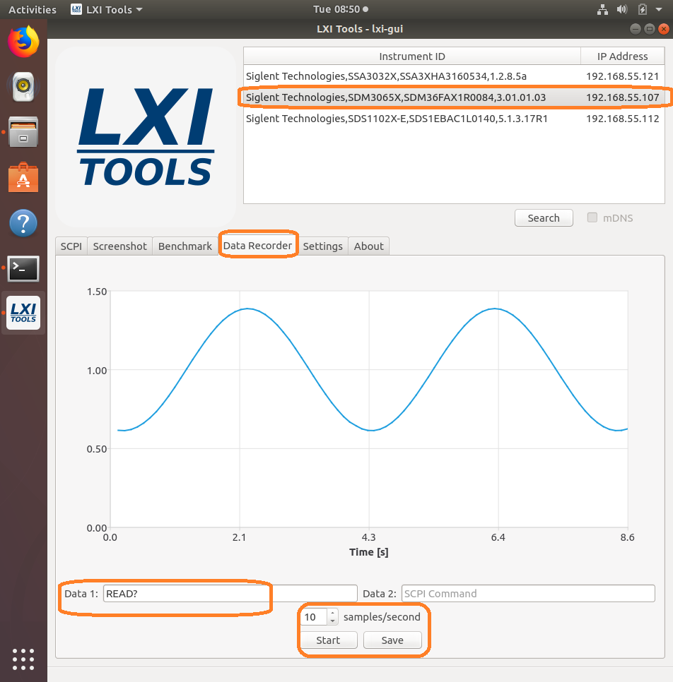
And the data:

- Settings: Configure the timeouts and other controls.

- About: Version info.
Verification of a LAN connection using Telnet
Automating a test can dramatically increase the productivity, throughput, and accuracy of a process. Automating a setup involves connecting a computer to the test instrumentation using a standard communications bus like USB or LAN and then utilizing code entered via a software layer (like LabVIEW, .NET, Python, etc..) to sequence the specific instrument commands and process data.
This process normally goes quite smoothly, but if there are problems, there are some basic troubleshooting steps that can help get your test up-and-running quickly.
In this note, we are going to show how to use Telnet to test the communications connection between an instrument and a remote computer using a LAN connection to ensure that it is working properly. Once the connection is verified, you can begin to work on the control software.
Telnet provides a means of communicating over a LAN connection. The Telnet client, run on a LAN connected computer, will create a login session on the instrument.
NOTE: The Telnet connection requires open sockets on the instrumentation. At this time, not all SIGLENT products feature open sockets. Check the product page FAQs or with your local SIGLENT support office for more information.
A connection, established between the computer and instrument, generates a user interface display screen with SCPI> prompts on the command line.
Using the Telnet protocol to send commands to the instrument is similar to communicating with USB. You establish a connection with the instrument and then send or receive information using SCPI commands. Communication is interactive: one command at a time.
The Windows operating systems use a command prompt style interface for the Telnet client.
STEPS
1. Power on and connect the instrument to the network via LAN
2. Verify that the Gateway, Subnet Mask, and IP address of the instrument are valid for the network you wish to use. This information is typically located in the System Information or IO menu. See the specific instrument user’s guide for more information on LAN settings.
3. On the computer, click Start > All Programs > Accessories > Command Prompt.
4. At the command prompt, type in telnet.
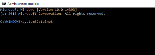
5. Press the Enter key. The Telnet display screen will be displayed.
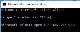
6. At the Telnet command line, type: open XXX.XXX.XXX.XXX 5024 where XXX.XXX.XXX.XXX is the instrument’s IP address and 5024 is the port. You should see a response similar to the following:
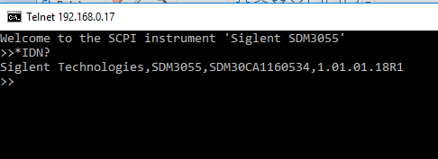
7. Now, you can enter any valid command for the specific instrument that you are controlling. See the specific programming guide for the instrument for more information.
This is especially helpful when you are planning a specific test sequence, the effect of delays/timing, or troubleshooting a command. You can send each command one-at-a-time and check the performance of the instrument.
*IDN? is a common identification string query (question or information request) that returns the information from the connected instrument

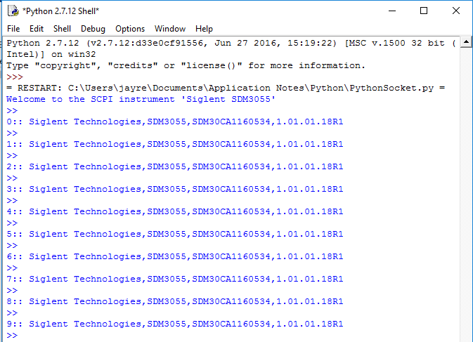
Programming Example: Open Socket LAN connection using Python
Automating a test can dramatically increase the productivity, throughput, and accuracy of a process. Automating a setup involves connecting a computer to the test instrumentation using a standard communications bus like USB or LAN and then utilising code entered via a software layer (like LabVIEW, .NET, Python, etc..) to sequence the specific instrument commands and process data.
In this note, we are going to show how to use Python to create a communications link between an instrument and a remote computer using a LAN connection. Once the connection is verified, you can begin to work on the control software.
NOTE: This example requires open sockets on the instrumentation. At this time, not all SIGLENT products feature open sockets. Check the product page FAQs or with your local SIGLENT support office for more information.
Python is an interpreted programming language that lets you work quickly and is very portable. Python has a low-level networking module that provides access to the socket interface. Python scripts can be written for sockets to do a variety of test and measurements tasks.
Here is a Python 2.7 script that opens a socket, sends a query and closes the socket. It performs this operation in a loop 10 times:
You can follow the instructions below to build your own example:
1. Power on and connect the instrument to the network via LAN
2. Verify that the Gateway, Subnet Mask, and IP address of the instrument are valid for the network you wish to use. This information is typically located in the System Information or IO menu. See the specific instrument user’s guide for more information on LAN settings.
3. Download python and your favourite python editor (I use IDLE):
https://docs.python.org/2/library/idle.html
Start your python editor:

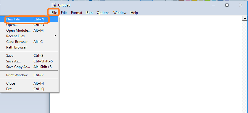
5. Open a new file by pressing File > New File.. and name the file
6. Copy and paste the code at the end of this note into the file editing window:
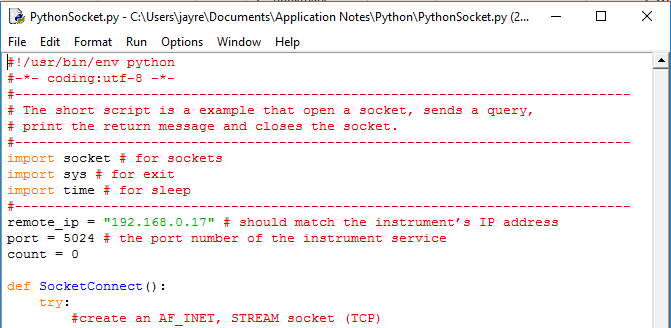
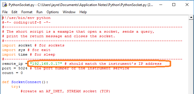
7. Change the IP address and port number so that they match the IP address and port for the instrument you wish to connect to:
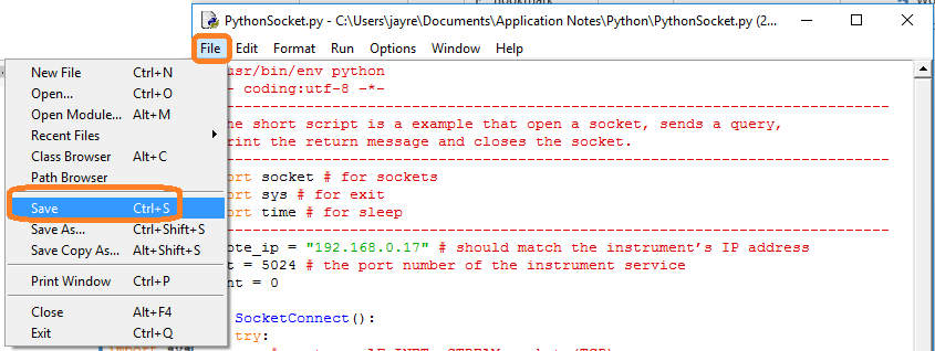
Save the file:
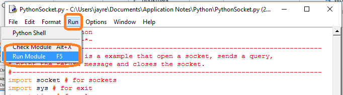
8. To Run, select Run and Run Module:
Programming Example: List connected VISA compatible resources using PyVISA
PyVISA is a software library that enables Python applications to communicate with resources (typically instruments) connected to a controlling computer using different buses, including: GPIB, RS-232, LAN, and USB.
This example scans and lists the available resources.
It requires PyVISA to be installed (see the PyVISA documentation for more information)
***
#Example that scans a computer for connected instruments that
#are compatible with the VISA communication protocol.
#
#The instrument VISA resource ID for each compatible instrument
#is then listed.
#
#
#Dependencies:
#Python 3.4 32 bit
#PyVisa 1.7
#
#Rev 1: 08302018 JCimport visa
def main():
rm = visa.ResourceManager()
print (rm.list_resources())if __name__==’__main__’:
main()
*****
Here is the code:
And here is the result of a scan:
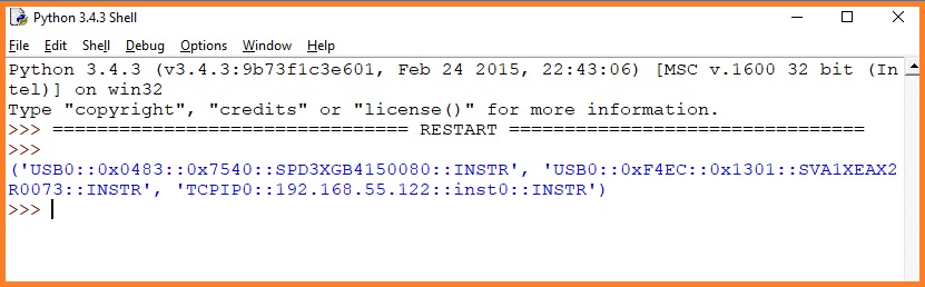
Each connected instrument returns a specific formatted string of characters called the VISA Resource ID.
The resource ID format is as follows:
‘Communication/Board Type (USB, GPIB, etc.)::Resource Information (Vendor ID, Product ID, Serial Number, IP address, etc..)::Resource Type’
In the response, each resource is separated by a comma. So, we have three resources listed in this example:
‘USB0::0x0483::0x7540::SPD3XGB4150080::INSTR’ – This is a power supply (SPD3X) connected via USB (USB0)
‘USB0::0xF4EC::0x1301::SVA1XEAX2R0073::INSTR’ – This is a vector network analyzer (SVA1X) connected via USB (USB0)
‘TCPIP0::192.168.55.122::inst0::INSTR’ – This is an instrument connected via LAN using a TCPIP connection at IP address 192.168.55.122

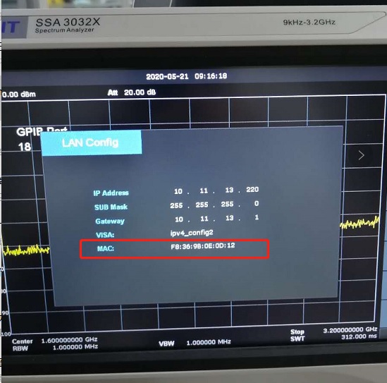
Where is the MAC address information for SSA3000X, SSA3000X Plus, SSA3000X-R, and SVA1000X?
The MAC address can be found on the LAN config interface.
Path: System–interface–LAN.
How do I pick the right spectrum analyser for my application?
The SIGLENT SSA3000X, SSA3000X Plus and SVA1000X products are based on a similar swept superheterodyne spectrum analyser platform and have very similar starting prices. There are quite a few similarities, but also a few differences that could affect the end results for particular applications. The table below compares the major specifications and the comparable options as they pertain to specific applications like VSWR.
SSA3000X Series SSA3000X Plus Series SVA1000X Series SSA3021X SSA3032X SSA3021X Plus SSA3032X Plus SVA1015X SVA1032X TG Standard Standard Standard SA Bandwidth 9 kHz – 2.1 GHz 9 kHz – 3.2 GHz 9 kHz – 2.1 GHz 9 kHz – 3.2 GHz 9 kHz – 1.5 GHz 9 kHz – 3.2 GHz VNA Bandwidth – – 10MHz – 1.5 GHz 100 kHz – 3.2 GHz VNA Calibration Kit – – F503ME DANL -151 dBm (RBW 10Hz) -161 dBm/Hz -156 dBm/Hz -161 dBm/Hz -161 dBm, Normalized to 1 Hz RBW 10 Hz – 1 MHz (1Hz settable) 1 Hz – 1 MHz 1 Hz – 1 MHz Phase Noise < -98 dBc/Hz@1 GHz, 10 kHz offset < -98 dBc/Hz@1 GHz, 10 kHz offset < -98 dBc/Hz@1 GHz, 10 kHz offset Options AMK/EMI/Refl* AMK/EMI/AMA/DMA AMK/EMI/AMA/DMA/DTF AMK details CHP/ACPR/TOI/OBW/Monitor CHP/ACPR/TOI/OBW/Monitor/Harmonic/CNR CHP/ACPR/TOI/OBW/Monitor/Harmonic/CNR AMA details – AM/FM AM/FM DMA details – ASK/FSK/PSK/QAM ASK/FSK/PSK/QAM EMI filter details 200 Hz, 9 kHz, 120 kHz 200 Hz, 9 kHz, 120 kHz, 1MHz 200 Hz, 9 kHz, 120 kHz, 1MHz Touch Screen – Touch Screen, Mouse & Keyboard, Webserver Touch Screen, Mouse & Keyboard, Webserver *Compatible with many commercially available return loss bridges/directional couplers
Additional SVA Features and Options
Still having trouble choosing? Here are some additional features and options that are exclusive to the SSA PLUS and SVA platforms that may help: Free Features:
- Touch screen control with shortcut widget
- Mouse/Keyboard support
- Easy web browser web control
- Power-On-Line – Instrument will automatically restart when power is restored to the mains power connection (power cord) when this feature is enabled.
Additional Options:
- AM/FM modulation analysis (SVA1000X-AMA. SSA3000XP-AMA) enables visualization of data encoded using AM/FM
- Digital modulation analysis (SVA1000X-DMA. SSA3000XP-DMA) enables visualization of data encoded using FSK/ASK
- Advanced measurement kit (SVA1000X-AMK, SSA3000XP-AMK) feature Harmonic and CNR measurements in addition to CHP/ACPR/TOI/OBW/Monitor.
- Mechanical calibration kit for VNA (F503ME)

Verification of a working remote communications connection using NI – MAX
Automating a test can dramatically increase the productivity, throughput, and accuracy of a process. Automating a setup involves connecting a computer to the test instrumentation using a standard communications bus like USB or LAN and then utilizing code entered via a software layer (like LabVIEW, .NET, Python, etc..) to sequence the specific instrument commands and process data.
This process normally goes quite smoothly, but if there are problems, there are some basic troubleshooting steps that can help get your test up-and-running quickly.
In this note, we are going to show how to use NI-MAX to test the communications connection between an instrument and a remote computer using both a USB and a LAN connection to ensure that they are working properly. Once the connection is verified, you can begin to work on the control software.
National Instruments Measurement and Automation Explorer (NI-MAX) is a free communications tool provided with NI’s VISA library.
You can learn more here: https://digital.ni.com/public.nsf/allkb/71544521BDE34FFB86256FCF005F4FB6
USB Connections
1. Power on and connect the instrument via USB cable to the computer. On a computer running Windows, the first time you connect the USB from an instrument should open a dialog box or show a notification of a new device being connected.
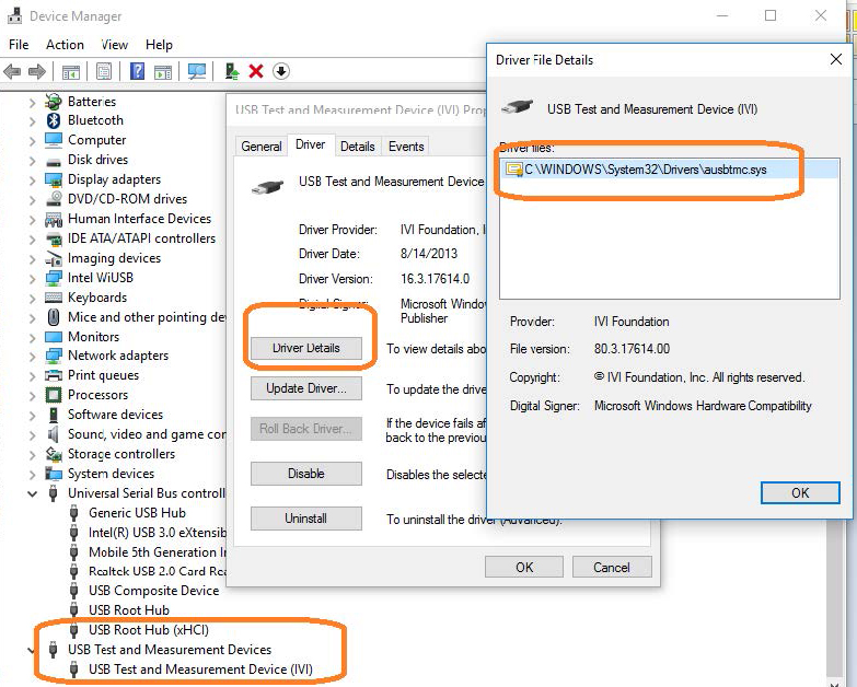
You can check the status of the USB connections by opening Device Manager located in the Control Panel menu of most Windows Operating systems and expanding the driver information as shown below in this Windows 10 example:
This indicates that the operating system recognizes the connected instrument as a test instrument.
If the device manager reports the USB connection as some other type of device (printer, camera, unknown, etc.), there is likely a problem linking the proper driver (ausbtmc.sys) to the instrument. One possible solution to this is to disable the driver, disconnect the USB cable, verify that ausbtmc.sys exists, and then reconnect the USB cable.
2. Run NI-MAX by left-clicking on the icon on the desktop or finding it via the start menu

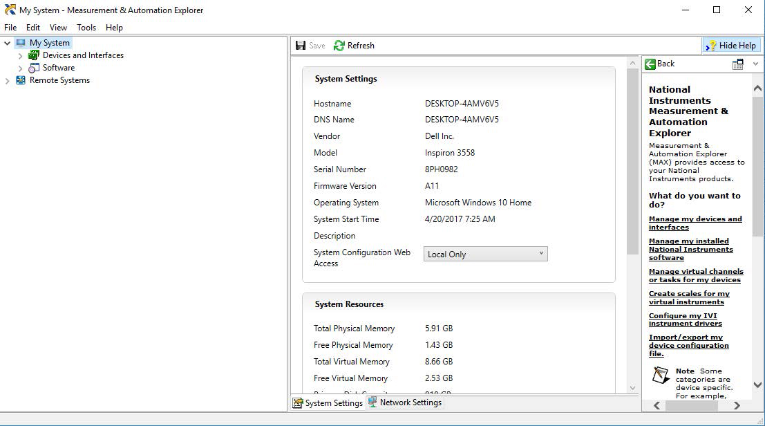
3. This will open the main window, as shown below:


4. Expand the “Devices and Interfaces” menu. You should see the instruments attached via USB with a brief description as shown for an SDS2000X oscilloscope below:
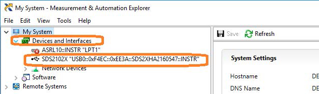
This indicates that a software application (NI-MAX) has correctly identified a test and measurement device (the oscilloscope) over the USB connection.
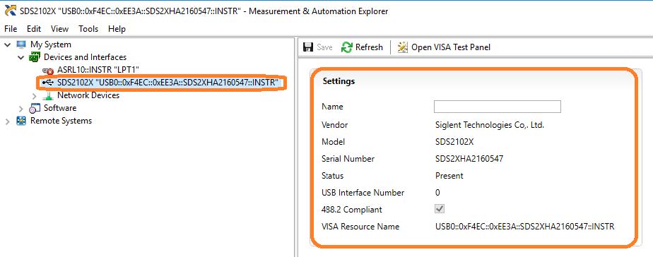
5. By left-clicking on the instrument, you can see additional information about it:
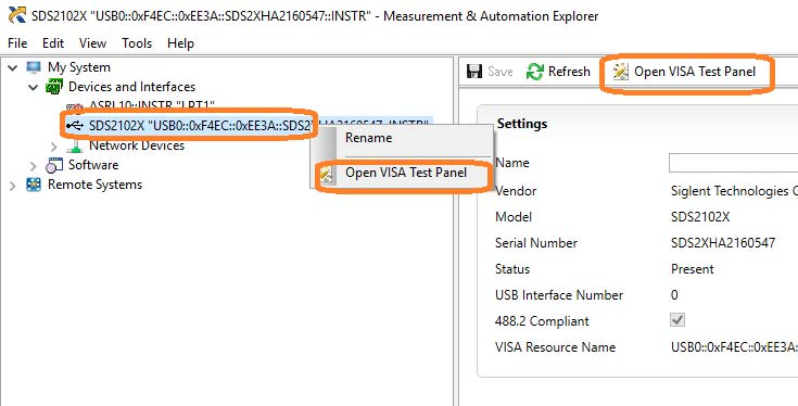
6. To further test the connection, right-click on the instrument and select Open VISA Test Panel or select it from the side bar:
The VISA Test Panel window shows some helpful information, including the instrument manufacturer, model, serial number, and the USB identifier (VISA Address) along the top.

7. Another useful item in the VISA Test Panel is the Input/Output function. This mode allows you to send specific instrument commands and receive instrument responses.
This is especially helpful when you are planning a specific test sequence, the effect of delays/timing, or troubleshooting a command. You can send each
command one-at-a-time and check the performance of the instrument.Select Input/Output > Basic I/O > and Enter the command in the text window:
– *IDN? is a common identification string query (question or information request) that returns the information from the connected instrument
– /n is a termination character that represents a new line. This is the standard termination character for SIGLENT instrumentation.
– Write will send the command to the instrument
– Read will pull data from the instrument
– Query will perform a read and then a write command to request and return data from the instrument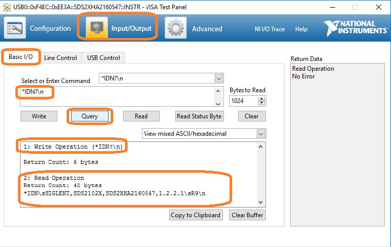
USB Checklist
– Is the USB port configured properly on the instrument? Some instruments feature USB ports that can be configured as TMC (Test and Measurement) or Printer communication ports. The USB port should be set to USBTMC or similar for remote control.
– Try a direct connection to the controlling computer. USB hubs or long connections may cause issues.
– Try a different USB cable. Connectors can go bad or prove to be faulty.
– Try a different USB port on the computer.
– On machines running Windows, check the Device Manager. Test instrumentation should appear as USB Test and Measurement Device (IVI) and use the AUSBTMC.SYS driverLan Connections
1. Power on and connect the instrument via LAN cable to a LAN network connected to the computer you wish to use.
You can check the status of the LAN connection by using a software tool like NMAP: https://nmap.org/

NMAP allows you to scan networks and identify IP addresses.
First, identify the LAN connection for the instrument. This is typically located in the System menu under IO or LAN settings.
Here is the IO information for an SDS2000X oscilloscope:
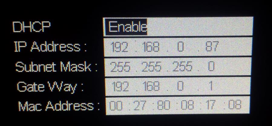
DHCP Enabled will automatically configure the instrument connection settings and apply a valid IP address. With DHCP enabled, the IP address may change over time. It is recommended to check the instrument IP address and then confirm that it is visible on the network using NMAP:
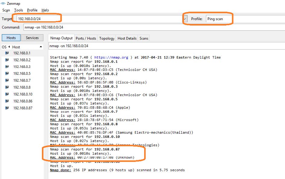
Here, we are performing a Ping (short scan to identify what IP addresses are being used) over the range of IP addresses that may match the instrument.
This can be performed by setting the target using the “/24” extension. This scans 24 bits For example, 192.168.10.0/24 would scan the 256 hosts between
192.168.10.0 and 192.168.10.255Here is more information from NMAP:
https://nmap.org/book/man-target-specification.htmlFor example, to ping all IP addresses that start with 192.168.0., set the target as follows:

Note the IP address and MAC address that identify your instrument.
2. Run NI-MAX by left-clicking on the icon on the desktop or finding it via the start menu

This will open the main window, as shown below:
3. Unlike USB, there is not an easy way to identify all of the instruments connected via LAN.
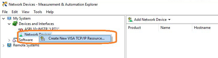
In many cases, you will have to manually add the LAN instrumentation. Recall from Step 2, our instrument IP address is 192.168.0.87
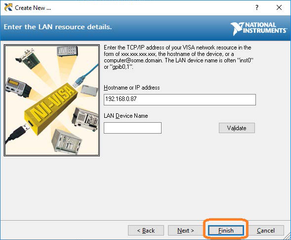
Right-click on Network Devices, and select Create New VISA TCP/IP Resource:
4. Select Manual Entry of LAN:

5. Enter the IP address and press Validate
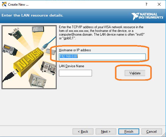
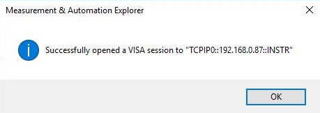
6. After successfully creating a TCP/IP connection, select finish
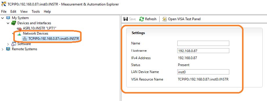
7. After the system updates it’s configuration, the instrument will appear in the Network Devices menu:
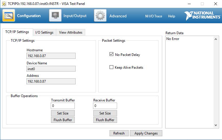
8. To further test the connection, right-click on the instrument and select Open VISA Test Panel or select it from the side bar:

The VISA Test Panel window shows some helpful information, including the TCP/IP identifier (VISA Address) along the top.
9. Another useful item in the VISA Test Panel is the Input/Output function. This mode allows you to send specific instrument commands and receive instrument responses.
This is especially helpful when you are planning a specific test sequence, the effect of delays/timing, or troubleshooting a command. You can send each command one-at-a-time and check the performance of the instrument.
Select Input/Output > Basic I/O > and Enter the command in the text window:
– *IDN? is a common identification string query (question or information request) that returns the information from the connected instrument
– /n is a termination character that represents a new line. This is the standard termination character for SIGLENT instrumentation.
– Write will send the command to the instrument
– Read will pull data from the instrument
– Query will perform a read and then a write command to request and return data from the instrument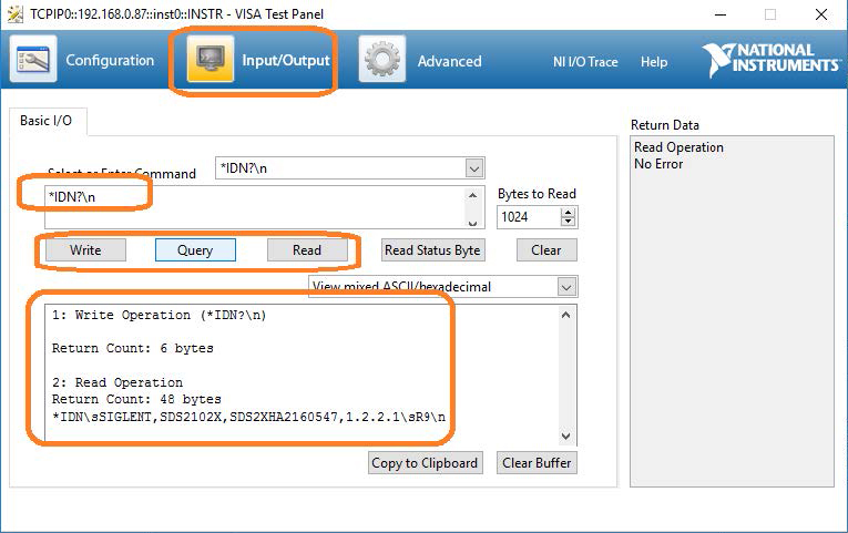
For more information, check SiglentAmerica.com, or contact your local Siglent office.
SDS FFT performance on low frequency signals
Like many modern oscilloscopes, the SIGLENT SDS series feature FFT math functions that calculate frequency information from the acquired voltage vs. time data. FFT stands for Fast Fourier Transform, and is a common method for determining the frequency content of a time-varying signal. Converting time domain data to the frequency domain makes measuring characteristics like phase noise and harmonics much easier. Oscilloscopes don’t have the dynamic range or sensitivity of a true spectrum analyzer, but these new designs can provide a fine level of detail that may be just enough for your application.
FFTs are commonly used on high frequencies, but they can also be used on signals with fairly low frequencies.
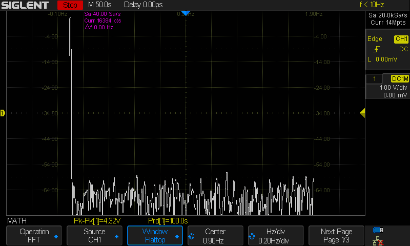
In this note, I am going to show the FFT performance of two series of our scopes by sourcing a 10 mHz (100 s period), 10 Vpp sine wave using a SIGLENT SDG805 Function Generator into Channel 1.
For those interested, here are the specs for the SDG805
SDS1000X/SDS2000X Series:
The SDS1000X and 2000X series feature an FFT function that uses up to 16 kpts of timebase data to calculate the frequency data and a timebase maximum of 50 s/div.
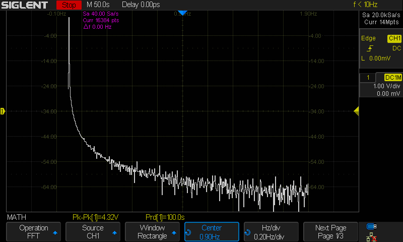
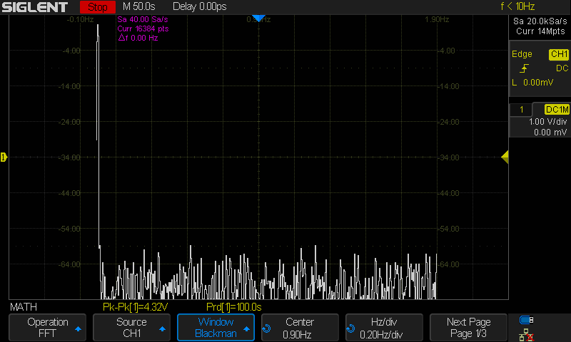
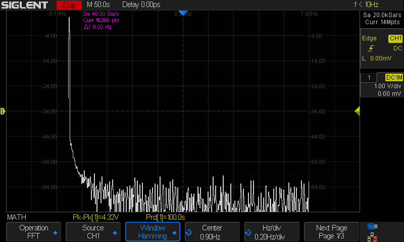
Here are the FFT results with the available window settings for a 10 mHz sinewave –
The scope can show a split timebase and FFT view:
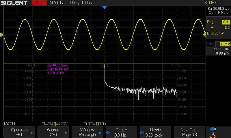
For the rest, I will use the exclusive FFT view.
Rectangle
Blackman
Hanning

Hamming
Flat Top
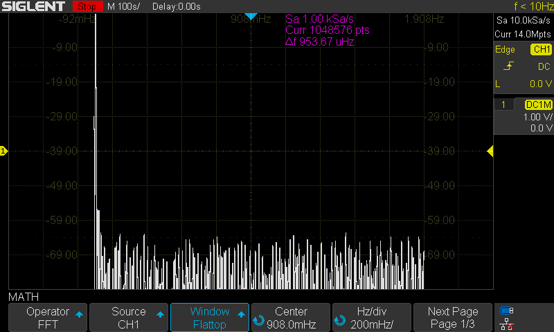
SDS1000X-E Series:
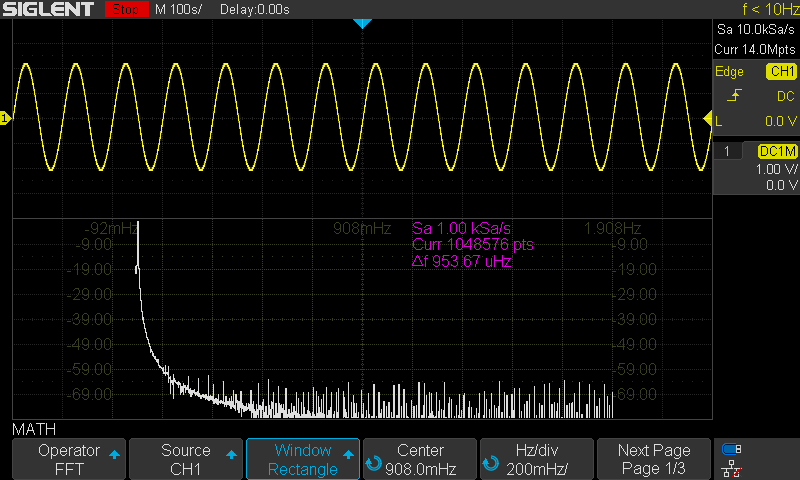
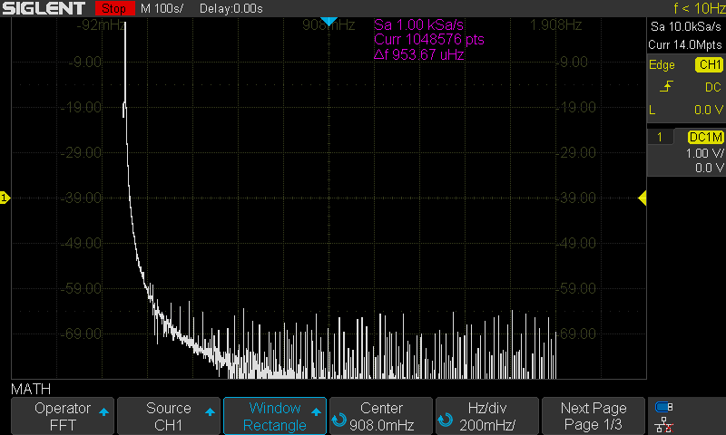
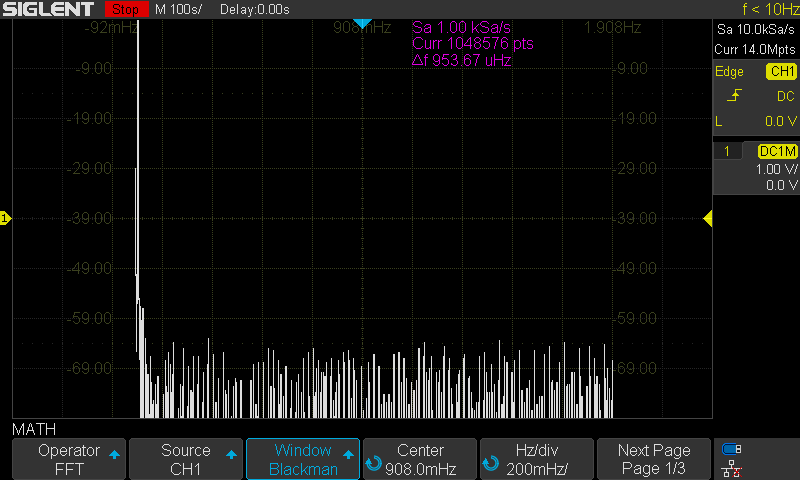
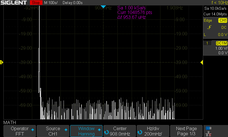
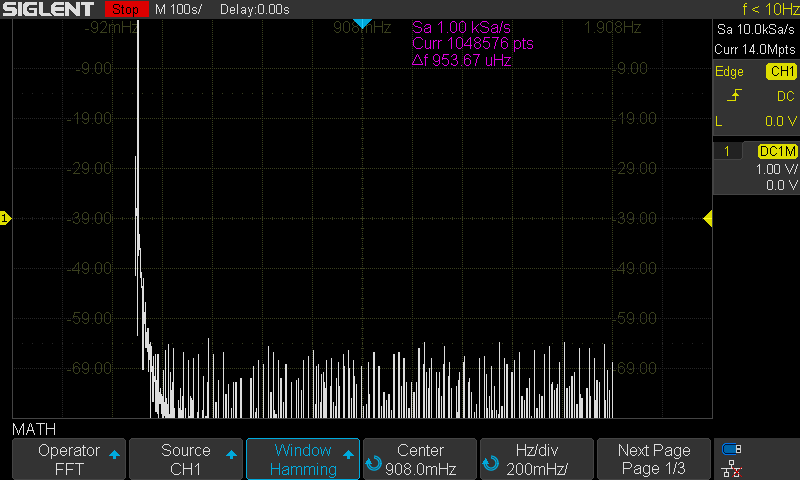
The SDS1000X-E series feature a new math co-processor that increases the maximum data depth of the FFT function to 1 Mpts. They also feature a timebase maximum of 100 s/div. These increases allow the X-E to have much finer timebase detail and to acquire useful data for even lower frequencies than many scopes on the market.
Here are the FFT results with the available window settings for a 10 mHz sinewave –
The scope can show a split timebase and FFT view:
For the rest, I will use the exclusive FFT view.
Rectangle
Blackman
Hanning
Hamming
Flat Top